Indicator Indifference, Indicator Sampling, and Structural Robustness

Why reflective indicators are not the construct — and why indicator choice still matters

Tommaso Feraco

Why this extra?

The core SEM assumptions:

latent paths are only as meaningful as the measurement model behind them
fit does not guarantee construct validity
structural interpretation should follow a defensible measurement model

This extra slows down on one deeper question:

If reflective indicators are meant to be manifestations of a construct, how much should the exact indicator set matter?

Here

what indicator indifference means
why it is a strong idea in psychology
why it matters for structural relations
an intelligence example
simulations on number of indicators and loading quality

Learning objectives

By the end of this extra, you should be able to:

explain the basic idea of indicator indifference under a reflective model
distinguish indicator indifference from measurement precision
explain why finite indicator choice can affect the stability of latent relations
interpret a simple simulation showing how number of indicators and loading size affect structural recovery
articulate why some indicators may be more central, more contaminated, or more auxiliary than others

The core idea

Reflective assumption

In a reflective measurement model:

the latent variable is conceptually prior to the indicators
item responses are treated as effects or manifestations of the latent variable
the construct is not identical to any one observed item

This is what makes latent-variable SEM more than a weighted sum-score exercise. It makes SEM theory-builder!

Indicator indifference: the strong reading

Strong interpretation

A strong reflective reading suggests:

If indicators are valid manifestations of the same latent variable, then the precise indicator set should not be the essence of the construct.

So, in principle different good indicators of the same construct

should support similar inferences about the latent variable
and should not radically change the substantive structural story

But psychology rarely gives us strict indifference

In applied psychology, indicators often differ in:

facet coverage
wording and method variance
task demands
contextual contamination
closeness to the construct of interest

So the practical question is usually not:

“Are indicators literally interchangeable?”

It is more often:

“How much do my conclusions depend on this particular sample of indicators?”

Note

In many areas, the facets included are directly used to define/label the upper-level constructs. When starting with an EFA this is necessary, but poses many limits…

Important distinction

Two nearby ideas

Indicator indifference: concerns whether the construct is conceptually tied to a particular indicator set
Measurement precision / indicator sampling: concerns how well a finite set of indicators helps us recover the latent variable and its relations

These are related, but they are not identical.

Why this matters for SEM

Structural relations are latent-level claims

In SEM, the substantive claim is usually about a relation such as:

\[ \eta_2 = \beta \eta_1 + \zeta \]

The claim is not primarily about one exact questionnaire form, but about a construct.

But in practice we only observe a finite, imperfect sample of indicators.

So structural estimates can depend on:

how many indicators we have
how strongly they load
whether one is weak or contaminated
whether the indicator set covers the construct well

Better wording than “good latent score”

SEM-friendly phrasing

Instead of asking:

“How many items do I need for a satisfying latent score?”

ask:

“How many and which indicators are needed to define the latent variable well enough that structural relations are estimated precisely and interpreted confidently?”

This is closer to how latent SEM actually works.

What would a robust result look like?

A practical criterion

If a reflective model is defensible, then:

swapping one reasonable indicator subset for another
or adding a few more good indicators

should not wildly change the latent regression or latent correlation.

If conclusions shift a lot, possibilities include:

weak measurement
too few indicators
multidimensionality
local dependence
cross-loadings
an underdefined construct

The case of ‘Intelligence’ (the g factor)

Intelligence research is a good illustration because:

many batteries aim to measure a broader construct such as general cognitive ability
but they include different mixtures of more central and more auxiliary tasks
and not all indicators look equally “close” to what people often mean by general reasoning

This makes it a useful teaching case for indicator centrality vs indicator contamination.

Intelligence example: central vs auxiliary indicators

Often treated as more central to reasoning

Matrix Reasoning
analogical / relational reasoning tasks
problem solving
tasks with strong fluid-reasoning content

Often more auxiliary or more contaminated

Processing speed tasks
tasks with strong motor demands
highly timed symbol substitution tasks
tasks where peripheral demands may contribute more strongly

The point

This does not mean processing speed is useless.

It means:

different indicators may not be equally pure manifestations of the same construct
batteries can still target “IQ” while mixing indicators with different degrees of centrality

Simulation section

Simulation plan

We simulate a simple SEM with a true latent relation:

\[ \eta_2 = 0.50 \eta_1 + \zeta \]

Then we vary:

the number of indicators per factor
the average loading strength
one problematic indicator

And we examine:

bias in the estimated path
standard errors / confidence intervals
stability across different indicator sets

Simulation 1: number of indicators

Design

two latent variables: eta1 and eta2
true path: beta = 0.50
equal loadings within a condition
sample size fixed, e.g. N = 400
number of indicators per factor: 2, 4, 8

Expectation:

with more good indicators, the structural estimate should usually become more precise
but “more” only helps if indicators are genuinely informative

Simulation code: one data-generating model

make_pop_model <- function(p = 4, lambda = 0.70, beta = 0.50) {

  x_names <- paste0("x", seq_len(p))
  y_names <- paste0("y", seq_len(p))

  x_load <- paste0(lambda, "*", x_names, collapse = " + ")
  y_load <- paste0(lambda, "*", y_names, collapse = " + ")

  resid_eta2 <- round(1 - beta^2, 3)

  paste(
    "eta1 =~", x_load,
    "\neta2 =~", y_load,
    "\neta2 ~", beta, "*eta1",
    "\neta1 ~~ 1*eta1",
    "\neta2 ~~", resid_eta2, "*eta2"
  )
}

make_fit_model <- function(p = 4) {
  x_names <- paste0("x", seq_len(p))
  y_names <- paste0("y", seq_len(p))

  paste(
    "eta1 =~", paste(x_names, collapse = " + "),
    "\neta2 =~", paste(y_names, collapse = " + "),
    "\neta2 ~ eta1"
  )
}

Simulation code: one replication

sim_once <- function(n = 400, p = 4, lambda = 0.70, beta = 0.50) {

  pop_model <- make_pop_model(p = p, lambda = lambda, beta = beta)
  fit_model <- make_fit_model(p = p)

  dat <- simulateData(pop_model, sample.nobs = n)
  fit <- sem(fit_model, data = dat)

  pe <- parameterEstimates(fit)

  out <- pe |>
    filter(lhs == "eta2", op == "~", rhs == "eta1") |>
    transmute(
      est = est,
      se = se,
      ci_low = ci.lower,
      ci_high = ci.upper
    )

  tibble(
    n = n,
    p = p,
    lambda = lambda,
    beta_true = beta,
    converged = lavInspect(fit, "converged"),
    est = out$est,
    se = out$se,
    ci_low = out$ci_low,
    ci_high = out$ci_high
  )
}

Simulation code: many replications

run_condition <- function(reps = 200, n = 400, p = 4, lambda = 0.70, beta = 0.50) {
  map_dfr(seq_len(reps), ~sim_once(n = n, p = p, lambda = lambda, beta = beta))
}

sim_n_indicators <- bind_rows(
  run_condition(reps = 1000, n = 400, p = 2, lambda = 0.70, beta = 0.50),
  run_condition(reps = 1000, n = 400, p = 4, lambda = 0.70, beta = 0.50),
  run_condition(reps = 1000, n = 400, p = 8, lambda = 0.70, beta = 0.50)
)

p	mean_est	sd_est	mean_se	coverage
2	0.5077023	0.1565695	0.1548884	0.925
4	0.4979402	0.0940654	0.0954821	0.940
8	0.5007732	0.0773124	0.0799038	0.950

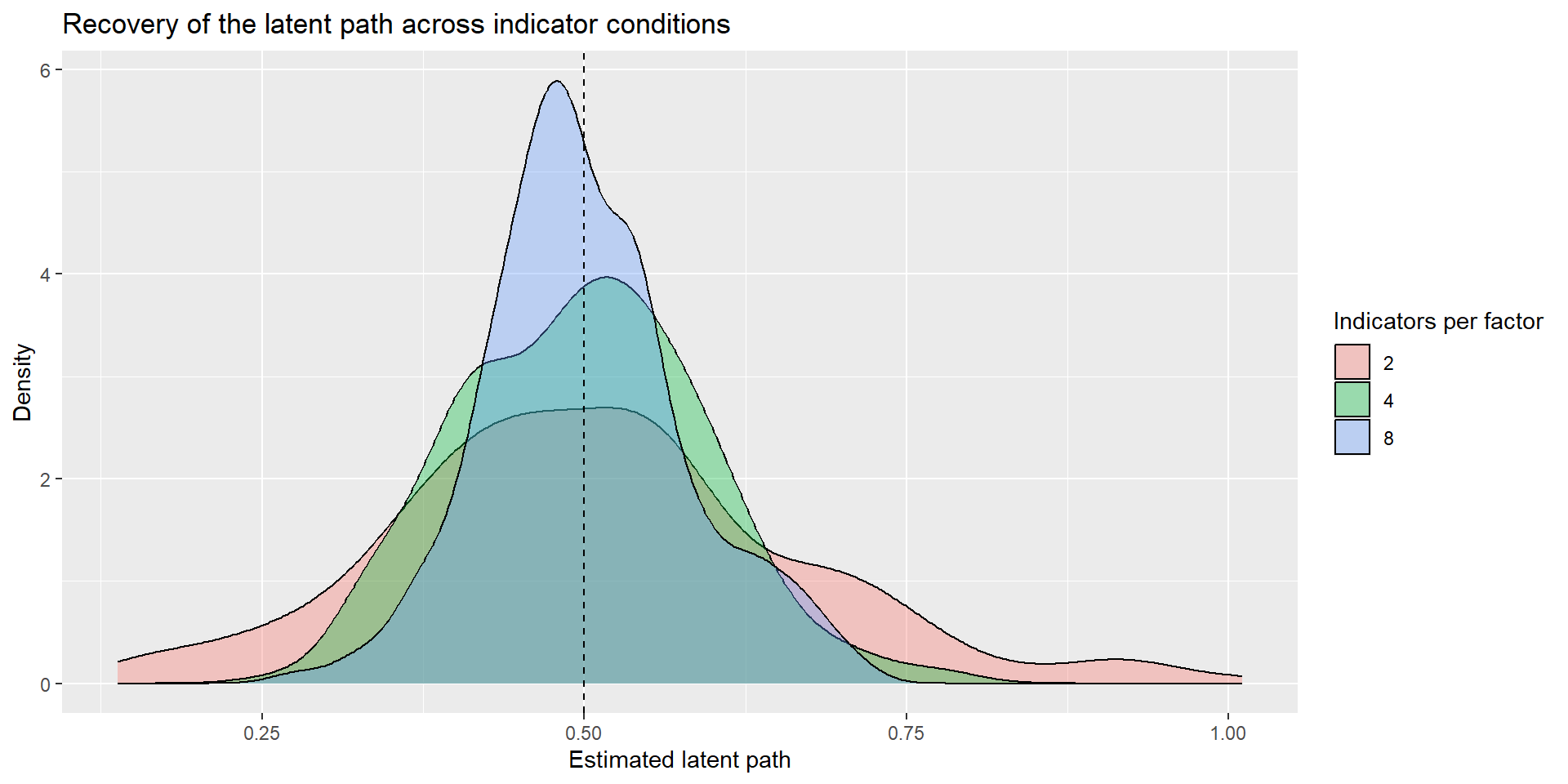
mean estimate: is it centered around the true path? (yes, all)

sampling variability: how much does the estimate move across replications? (less with more)

average SE / CI width: how precisely is the path estimated? (better with more)

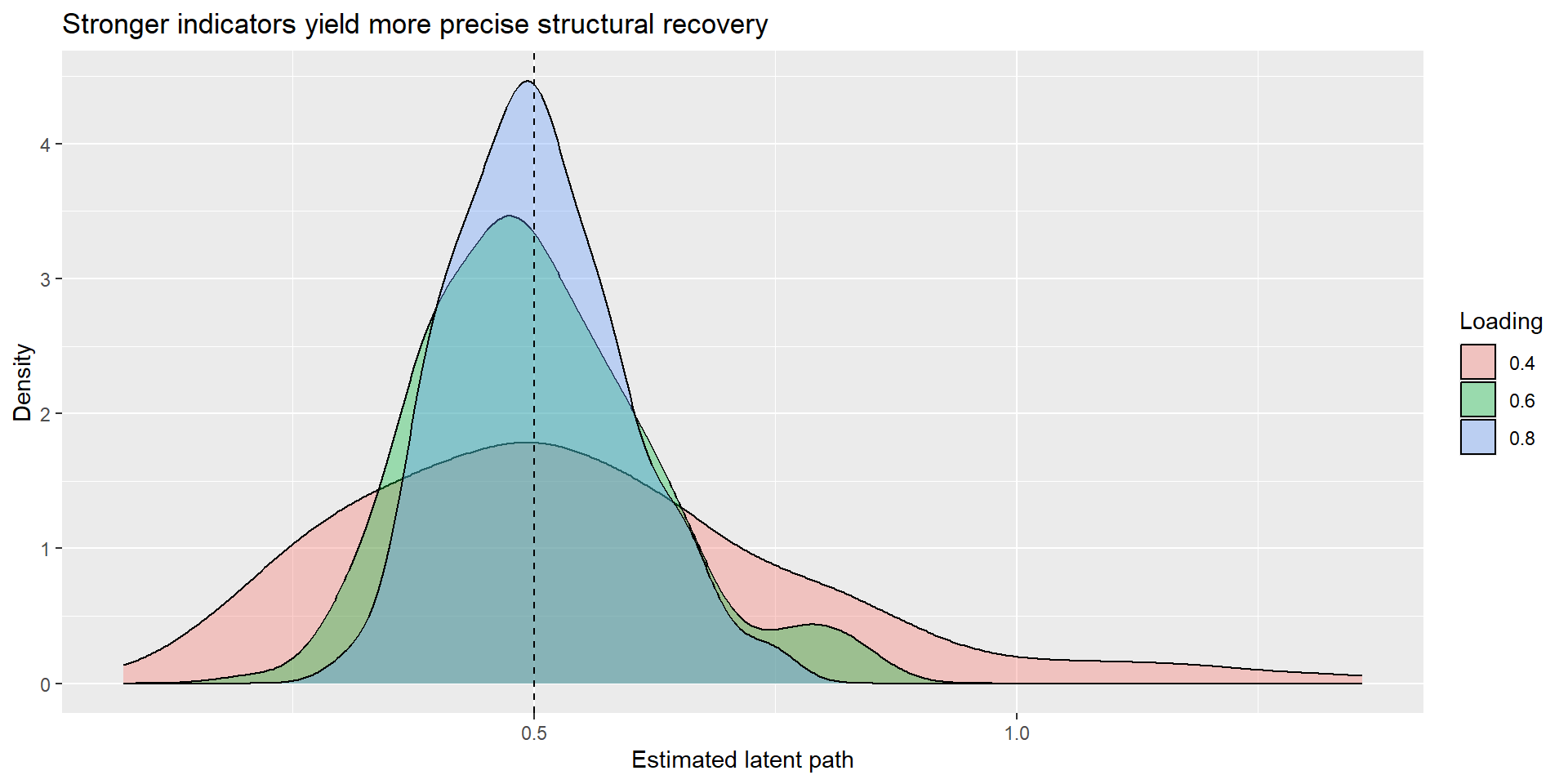
Simulation 2: loading strength

Design

Now hold the number of indicators constant and vary loading quality:

p = 4
loadings = .40, .60, .80

Expectation:

stronger loadings should generally improve the precision of the latent path estimate
the issue is not just how many indicators we have, but how informative they are

Simulation code: varying loading size

sim_loading <- bind_rows(
  run_condition(reps = 1000, n = 400, p = 4, lambda = 0.40, beta = 0.50),
  run_condition(reps = 1000, n = 400, p = 4, lambda = 0.60, beta = 0.50),
  run_condition(reps = 1000, n = 400, p = 4, lambda = 0.80, beta = 0.50)
)

lambda	m_est	sd_est	m_se	coverage
0.4	0.54	0.24	0.22	0.90
0.6	0.50	0.12	0.12	0.92
0.8	0.50	0.09	0.08	0.94

Why “more items” is not the whole story

Quantity vs quality

Ten indicators are not automatically better than three.

More items only help when they are:

relevant to the construct
sufficiently strong
not dominated by method effects
not merely redundant clones
not obviously contaminated by different latent causes

So the practical lesson is:

More good indicators help.
More weak or contaminated indicators may not.

Optional extension: one problematic indicator

A simple extension

You can extend the simulation by making one indicator weaker or contaminated.

Examples:

one item with loading .20
one cross-loading indicator
one pair of locally dependent indicators

Question:

Does the latent path stay stable when one problematic indicator enters the measurement model?

That is often more interesting than asking only whether the overall fit stays acceptable.

Pitfall callout

Pitfall

Do not conclude:

“two indicators are always enough”
“more items always solve the problem”
“good fit proves indicator indifference”
“a latent variable is automatically transportable across item sets”

The bigger lesson is about robustness of interpretation, not just identification or model fit.

Exercises

Suggested short tasks

Run Simulation 1 with N = 200, 400, and 800.
How much does sample size interact with number of indicators?
Repeat Simulation 2 with unequal loadings, e.g. .80, .80, .50, .30.
What happens to the path estimate and its standard error?
Add one weak or cross-loading indicator.
Does the latent path change meaningfully?
Try a sum-score regression using the same generated indicators.
Compare it with the latent SEM estimate.

Three things to remember

3 take-home messages

Indicator indifference is a strong reflective idea, not a routine empirical fact in psychology.
Finite indicator choice still matters because structural recovery depends on indicator quality, quantity, and construct coverage.
Robust latent relations should not be overly item-bound: if a reasonable indicator swap changes the story, revisit the measurement model before interpreting the path.

Indicator Indifference, Indicator Sampling, and Structural Robustness

Why this extra?

Learning objectives

The core idea

Reflective assumption

Indicator indifference: the strong reading

Strong interpretation

But psychology rarely gives us strict indifference

Important distinction

Two nearby ideas

Why this matters for SEM

Structural relations are latent-level claims

Better wording than “good latent score”

SEM-friendly phrasing

What would a robust result look like?

A practical criterion

The case of ‘Intelligence’ (the g factor)

Intelligence example: central vs auxiliary indicators

Often treated as more central to reasoning

Often more auxiliary or more contaminated

The point

Simulation section

Simulation plan

Simulation 1: number of indicators

Design

Simulation code: one data-generating model

Simulation code: one replication

Simulation code: many replications

Simulation 2: loading strength

Design

Simulation code: varying loading size

Why “more items” is not the whole story

Optional extension: one problematic indicator

Pitfall callout

Exercises

Suggested short tasks

Three things to remember

3 take-home messages

Further reading

Suggested follow-up

References