Lab 06 — Missing data, FIML, MI, and robust estimation

Author

Tommaso Feraco

Goals

By the end of this lab, you can:

Diagnose what kind of missingness you likely have (MCAR/MAR/MNAR)
Fit the same SEM under different defensible choices (listwise vs FIML; ML vs MLR)
Run multiple imputation (MI) and compare with FIML
Write a minimal, defensible reporting paragraph for a SEM with missing and non-normal data

Setup

Show code

library(lavaan)

# Optional packages (install if needed)
# install.packages(c("semTools", "mice"))
library(semTools)
library(mice)

set.seed(1234)

Simulate a “messy but realistic” dataset

We reuse the same model as in Lesson 6 (measurement + structural), then we add:

skewness (monotone transforms of some indicators)
heavy tails/outliers (a small proportion of extreme values)
MAR missingness (missingness depends on an observed proxy)

Show code

simulate_sem_data <- function(N = 600, seed = 1234,
                              add_skew = TRUE,
                              add_outliers = TRUE) {
  set.seed(seed)

  model_pop <- "
  # Measurement
  peer  =~ 0.80*p1 + 0.70*p2 + 0.60*p3 + 0.70*p4
  media =~ 0.70*m1 + 0.80*m2 + 0.60*m3 + 0.70*m4
  comp  =~ 0.70*c1 + 0.70*c2 + 0.60*c3
  eat   =~ 0.70*e1 + 0.60*e2

  # Structural
  comp ~ 0.40*peer + 0.50*media
  eat  ~ 0.35*comp
  "

  dat <- simulateData(model_pop, sample.nobs = N)

  if (add_skew) {
    skew_vars <- c("p1","p2","m1","m2","c1")
    for (v in skew_vars) dat[[v]] <- exp(dat[[v]] / 2)
  }

  if (add_outliers) {
    set.seed(seed)
    ix <- sample(seq_len(N), size = round(0.03 * N))  # ~3% outliers
    dat$m4[ix] <- dat$m4[ix] + rnorm(length(ix), mean = 0, sd = 4)
    dat$c3[ix] <- dat$c3[ix] + rnorm(length(ix), mean = 0, sd = 4)
  }

  dat
}

make_missing_mar <- function(dat, prop = 0.20, seed = 1234,
                             vars = c("e1","m3")) {
  set.seed(seed)

  # Observed proxy for the latent 'peer' factor (think: sum score, previous wave, etc.)
  peer_obs <- rowMeans(dat[, c("p1","p2","p3","p4")], na.rm = TRUE)

  # Base MAR mechanism: higher peer_obs -> higher missingness probability
  p_base <- plogis(as.numeric(scale(peer_obs)))  # in (0,1), mean ~ 0.5

  # Calibrate to hit approx prop missing (cap to avoid p > 1)
  k <- min(0.95, prop / mean(p_base))
  p_miss <- pmin(p_base * k, 0.95)

  miss <- runif(nrow(dat)) < p_miss

  for (v in vars) dat[[v]][miss] <- NA

  attr(dat, "missing_mechanism") <- list(type = "MAR", prop_target = prop, vars = vars)
  dat
}

# Build the dataset used throughout the lab
dat <- simulate_sem_data(N = 600, seed = 1234)
dat <- make_missing_mar(dat, prop = 0.20, seed = 1234)

round(colMeans(is.na(dat)), 3)

   p1    p2    p3    p4    m1    m2    m3    m4    c1    c2    c3    e1    e2 
0.000 0.000 0.000 0.000 0.000 0.000 0.175 0.000 0.000 0.000 0.000 0.175 0.000

Exercise 1 — Diagnose missingness (MCAR / MAR / MNAR)

Task

Compute the percent missing for each variable.
Inspect missingness patterns (are some variables missing together?).
Test whether missingness is related to observed variables (evidence consistent with MAR).

Suggested tools: colMeans(is.na(.)), md.pattern() (mice), and simple regressions.

Show code

# 1) % missing per variable
round(colMeans(is.na(dat)), 3)

   p1    p2    p3    p4    m1    m2    m3    m4    c1    c2    c3    e1    e2 
0.000 0.000 0.000 0.000 0.000 0.000 0.175 0.000 0.000 0.000 0.000 0.175 0.000

Show code

# 2) Missingness patterns
md.pattern(dat)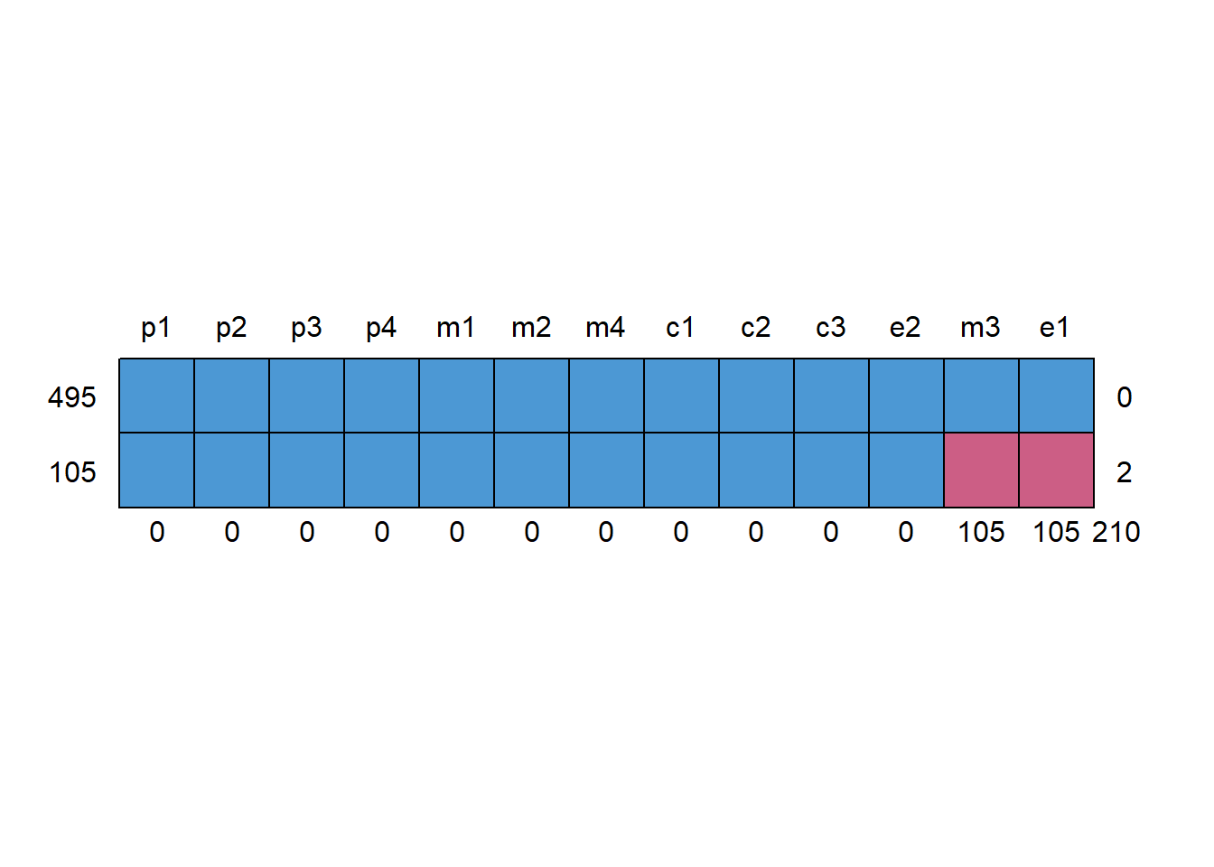

    p1 p2 p3 p4 m1 m2 m4 c1 c2 c3 e2  m3  e1    
495  1  1  1  1  1  1  1  1  1  1  1   1   1   0
105  1  1  1  1  1  1  1  1  1  1  1   0   0   2
     0  0  0  0  0  0  0  0  0  0  0 105 105 210

Show code

# 3) Is missingness related to observed information?
# Example: create a missingness indicator for e1 and see if it relates to peer_obs
peer_obs <- rowMeans(dat[, c("p1","p2","p3","p4")], na.rm = TRUE)
r_e1 <- as.integer(is.na(dat$e1))

summary(lm(r_e1 ~ peer_obs))


Call:
lm(formula = r_e1 ~ peer_obs)

Residuals:
     Min       1Q   Median       3Q      Max 
-0.47741 -0.20106 -0.14282 -0.07445  0.99382 

Coefficients:
            Estimate Std. Error t value Pr(>|t|)    
(Intercept)  0.10767    0.02008   5.363 1.17e-07 ***
peer_obs     0.11724    0.02283   5.136 3.81e-07 ***
---
Signif. codes:  0 '***' 0.001 '**' 0.01 '*' 0.05 '.' 0.1 ' ' 1

Residual standard error: 0.3725 on 598 degrees of freedom
Multiple R-squared:  0.04224,   Adjusted R-squared:  0.04064 
F-statistic: 26.37 on 1 and 598 DF,  p-value: 3.812e-07

Exercise 2 — Same SEM: listwise vs FIML

We now fit the same model under two missing-data choices.

Show code

model_sem <- "
# Measurement
peer  =~ p1 + p2 + p3 + p4
media =~ m1 + m2 + m3 + m4
comp  =~ c1 + c2 + c3
eat   =~ e1 + e2

# Structural
comp ~ peer + media
eat  ~ comp
"

key_paths <- function(fit) {
  pe <- parameterEstimates(fit)
  pe <- pe[pe$op == "~" & pe$lhs %in% c("comp","eat"), ]
  pe[pe$rhs %in% c("peer","media","comp"),
     c("lhs","op","rhs","est","se","z","pvalue")]
}

Task

Fit the model with default missing handling (listwise deletion).
Fit the model with missing = "fiml".
Compare (a) sample size used, (b) fit indices, (c) the three structural paths.

Show code

# 1) Listwise (default)
fit_list <- sem(model_sem, data = dat)

# 2) FIML
fit_fiml <- sem(model_sem, data = dat, missing = "fiml")

# 3) Compare fit
fitMeasures(fit_list, c("nobs","chisq","df","cfi","tli","rmsea","srmr"))

 chisq     df    cfi    tli  rmsea   srmr 
56.563 61.000  1.000  1.008  0.000  0.030

Show code

fitMeasures(fit_fiml, c("nobs","chisq","df","cfi","tli","rmsea","srmr"))

 chisq     df    cfi    tli  rmsea   srmr 
55.633 61.000  1.000  1.009  0.000  0.027

Show code

# Compare key paths
rbind(
  listwise = key_paths(fit_list),
  fiml     = key_paths(fit_fiml)
)

             lhs op   rhs   est    se     z pvalue
listwise.14 comp  ~  peer 0.387 0.103 3.738  0.000
listwise.15 comp  ~ media 0.428 0.093 4.609  0.000
listwise.16  eat  ~  comp 0.428 0.124 3.447  0.001
fiml.14     comp  ~  peer 0.412 0.089 4.605  0.000
fiml.15     comp  ~ media 0.451 0.085 5.283  0.000
fiml.16      eat  ~  comp 0.427 0.122 3.503  0.000

Exercise 3 — Robust estimation: ML vs MLR (with FIML)

Because we introduced skewness and heavy tails, normal-theory SEs can be too optimistic.

Task

Fit with estimator = "MLR" and missing = "fiml".
Compare key paths against ML+FIML.
Identify which part changes the most: point estimates or SE/p-values?

Show code

fit_mlr <- sem(model_sem, data = dat,
               missing = "fiml",
               estimator = "MLR")

# Compare fit measures (note: robust/scaled test statistic for MLR)
fitMeasures(fit_fiml, c("chisq","df","cfi","tli","rmsea","srmr"))

 chisq     df    cfi    tli  rmsea   srmr 
55.633 61.000  1.000  1.009  0.000  0.027

Show code

fitMeasures(fit_mlr,  c("chisq","df","cfi","tli","rmsea","srmr"))

 chisq     df    cfi    tli  rmsea   srmr 
55.633 61.000  1.000  1.009  0.000  0.027

Show code

# Compare paths
rbind(
  fiml_ML  = key_paths(fit_fiml),
  fiml_MLR = key_paths(fit_mlr)
)

             lhs op   rhs   est    se     z pvalue
fiml_ML.14  comp  ~  peer 0.412 0.089 4.605  0.000
fiml_ML.15  comp  ~ media 0.451 0.085 5.283  0.000
fiml_ML.16   eat  ~  comp 0.427 0.122 3.503  0.000
fiml_MLR.14 comp  ~  peer 0.412 0.091 4.506  0.000
fiml_MLR.15 comp  ~ media 0.451 0.146 3.082  0.002
fiml_MLR.16  eat  ~  comp 0.427 0.122 3.505  0.000

Exercise 4 — Stress test: increase missingness to ~40%

Task

Re-generate the dataset with ~40% MAR missingness on e1 and m3.
Repeat Exercise 2–4.
In 2–3 sentences: at what point does your inference become fragile?

Show code

dat40 <- simulate_sem_data(N = 600, seed = 2222)
dat40 <- make_missing_mar(dat40, prop = 0.40, seed = 2222)

round(colMeans(is.na(dat40)), 3)

   p1    p2    p3    p4    m1    m2    m3    m4    c1    c2    c3    e1    e2 
0.000 0.000 0.000 0.000 0.000 0.000 0.402 0.000 0.000 0.000 0.000 0.402 0.000

Show code

fit_list40 <- sem(model_sem, data = dat40)
fit_fiml40 <- sem(model_sem, data = dat40, missing = "fiml")
fit_mlr40  <- sem(model_sem, data = dat40, missing = "fiml", estimator = "MLR")

rbind(
  listwise = key_paths(fit_list40),
  fiml_ML  = key_paths(fit_fiml40),
  fiml_MLR = key_paths(fit_mlr40)
)

             lhs op   rhs   est    se     z pvalue
listwise.14 comp  ~  peer 0.341 0.103 3.295  0.001
listwise.15 comp  ~ media 0.589 0.117 5.045  0.000
listwise.16  eat  ~  comp 0.799 0.209 3.822  0.000
fiml_ML.14  comp  ~  peer 0.279 0.073 3.807  0.000
fiml_ML.15  comp  ~ media 0.517 0.094 5.513  0.000
fiml_ML.16   eat  ~  comp 0.660 0.172 3.832  0.000
fiml_MLR.14 comp  ~  peer 0.279 0.071 3.930  0.000
fiml_MLR.15 comp  ~ media 0.517 0.109 4.754  0.000
fiml_MLR.16  eat  ~  comp 0.660 0.171 3.850  0.000

Exercise 5 — (Optional) MNAR simulation: when FIML/MI can still be biased

This is a didactic stress test: we create missingness depending on the (unobserved) value itself.

Show code

make_missing_mnar <- function(dat, prop = 0.20, seed = 999, var = "e1") {
  set.seed(seed)

  p_base <- plogis(as.numeric(scale(dat[[var]])))  # depends on the value itself (MNAR)
  k <- min(0.95, prop / mean(p_base))
  p_miss <- pmin(p_base * k, 0.95)

  miss <- runif(nrow(dat)) < p_miss
  dat[[var]][miss] <- NA

  attr(dat, "missing_mechanism") <- list(type = "MNAR", prop_target = prop, vars = var)
  dat
}

dat_mnar <- simulate_sem_data(N = 600, seed = 3333)
dat_mnar <- make_missing_mnar(dat_mnar, prop = 0.25, seed = 3333, var = "e1")
round(colMeans(is.na(dat_mnar)), 3)

   p1    p2    p3    p4    m1    m2    m3    m4    c1    c2    c3    e1    e2 
0.000 0.000 0.000 0.000 0.000 0.000 0.000 0.000 0.000 0.000 0.000 0.228 0.000

Show code

fit_fiml_mnar <- sem(model_sem, data = dat_mnar, missing = "fiml", estimator = "MLR")
key_paths(fit_fiml_mnar)

    lhs op   rhs   est    se     z pvalue
14 comp  ~  peer 0.223 0.069 3.255  0.001
15 comp  ~ media 0.471 0.121 3.881  0.000
16  eat  ~  comp 0.789 0.155 5.091  0.000

Exercise 6 — Reporting paragraph (deliverable)

Task

Write a short paragraph (6–10 lines) that includes:

estimator (MLR vs ML)
missing handling (FIML vs MI)
model fit: χ²(df), CFI, TLI, RMSEA (+ CI), SRMR
1–2 key substantive paths with standardized estimates (and CI/p)

You can start from this scaffold:

The SEM was estimated in lavaan using ______ with ______ for missing data under a ______ assumption. Model fit was evaluated using ______. The paths from ______ to ______ and from ______ to ______ were ______ (β = , SE = , p = ). Sensitivity checks comparing ____ vs ______ indicated that ______.

Show code

# Helper: grab the key fit measures for your chosen final model
final_fit <- fit_mlr  # change if you want MI (fit_mi) or another choice
fitMeasures(final_fit, c("chisq","df","cfi","tli","rmsea","srmr"))

 chisq     df    cfi    tli  rmsea   srmr 
55.633 61.000  1.000  1.009  0.000  0.027

Common mistakes checklist

Treating FIML as “imputation” (it isn’t; it is likelihood-based under MAR)
Reporting ML χ² after estimating MLR (mixing runs)
Declaring “MNAR” without evidence (usually we only have plausibility arguments)
Using MI without thinking about the imputation model (auxiliaries matter)
Overinterpreting fit indices with messy data (use global + local diagnostics)

Reproducibility

Show code

sessionInfo()

R version 4.5.1 (2025-06-13 ucrt)
Platform: x86_64-w64-mingw32/x64
Running under: Windows 11 x64 (build 26100)

Matrix products: default
  LAPACK version 3.12.1

locale:
[1] LC_COLLATE=Italian_Italy.utf8  LC_CTYPE=Italian_Italy.utf8   
[3] LC_MONETARY=Italian_Italy.utf8 LC_NUMERIC=C                  
[5] LC_TIME=Italian_Italy.utf8    

time zone: Europe/Rome
tzcode source: internal

attached base packages:
[1] stats     graphics  grDevices utils     datasets  methods   base     

other attached packages:
[1] mice_3.18.0    semTools_0.5-7 lavaan_0.6-19 

loaded via a namespace (and not attached):
 [1] shape_1.4.6.1      xfun_0.52          htmlwidgets_1.6.4  lattice_0.22-7    
 [5] quadprog_1.5-8     vctrs_0.6.5        tools_4.5.1        Rdpack_2.6.4      
 [9] generics_0.1.4     stats4_4.5.1       parallel_4.5.1     sandwich_3.1-1    
[13] tibble_3.3.0       pan_1.9            pkgconfig_2.0.3    jomo_2.7-6        
[17] Matrix_1.7-3       lifecycle_1.0.4    compiler_4.5.1     mnormt_2.1.1      
[21] codetools_0.2-20   htmltools_0.5.8.1  yaml_2.3.10        glmnet_4.1-10     
[25] pillar_1.11.0      nloptr_2.2.1       tidyr_1.3.1        MASS_7.3-65       
[29] reformulas_0.4.1   iterators_1.0.14   rpart_4.1.24       boot_1.3-31       
[33] multcomp_1.4-28    foreach_1.5.2      mitml_0.4-5        nlme_3.1-168      
[37] tidyselect_1.2.1   digest_0.6.37      mvtnorm_1.3-3      dplyr_1.1.4       
[41] purrr_1.0.4        splines_4.5.1      fastmap_1.2.0      grid_4.5.1        
[45] cli_3.6.5          magrittr_2.0.3     survival_3.8-3     broom_1.0.8       
[49] pbivnorm_0.6.0     TH.data_1.1-3      backports_1.5.0    estimability_1.5.1
[53] rmarkdown_2.29     emmeans_1.11.1     nnet_7.3-20        lme4_1.1-37       
[57] zoo_1.8-14         coda_0.19-4.1      evaluate_1.0.4     knitr_1.50        
[61] rbibutils_2.3      rlang_1.1.6        Rcpp_1.0.14        xtable_1.8-4      
[65] glue_1.8.0         rstudioapi_0.17.1  minqa_1.2.8        jsonlite_2.0.0    
[69] R6_2.6.1

Goals

Setup

Simulate a “messy but realistic” dataset

Exercise 1 — Diagnose missingness (MCAR / MAR / MNAR)

Exercise 2 — Same SEM: listwise vs FIML

Exercise 3 — Robust estimation: ML vs MLR (with FIML)

Exercise 4 — Stress test: increase missingness to ~40%

Exercise 5 — (Optional) MNAR simulation: when FIML/MI can still be biased

Exercise 6 — Reporting paragraph (deliverable)

Common mistakes checklist

Reproducibility

References