SEM foundations: language, workflow, first lavaan steps

Structural Equation Modeling (SEM)

Tommaso Feraco

Today in the workflow

Specify → Identify → Estimate → Evaluate → Revise/Report

Today: SEM language + diagram grammar + the workflow, then first translation to lavaan.
Next (02): path analysis & mediation (indirect effects, equivalence, interpretation).

Learning objectives

By the end of this session you should be able to:

• Translate a verbal hypothesis into a diagram
• Use the basic SEM “grammar” (variables, errors, arrows, covariances)
• Explain the SEM workflow: Specify → Identify → Estimate → Evaluate → Revise/Report
• Write and run a minimal model in lavaan (and read the key parts of the output)

A quick motivation: “how do you fit these?”

SEM = Structural Equation Modeling

A family of models that lets you:

• represent hypotheses as a system of relations

  1. postulate a data-generating model
  2. evaluate whether this model fits the data or not

• work with measurement error (explicitly)

• model means and covariances implied by your theory

it includes path-analysis, causal models, factorial models, measurement models, Latent Growth Models, but even regressions, ANOVAs, t-tests could be considered particular cases of SEM.

• model latent variables (e.g., ‘invisible constructs’)
• test indirect, moderated, and reciprocal effects
• make diagrams (or PAINTINGS if theory is weak!)

network models are better if you want good paintings with no theory.

Variance–covariance matrices (the “currency”)

options(digits = 2)
cov(PoliticalDemocracy[1:7])

    y1   y2   y3   y4  y5   y6   y7
y1 6.9  6.3  5.8  6.1 5.1  5.7  5.8
y2 6.3 15.6  5.8  9.5 5.6  9.4  7.5
y3 5.8  5.8 10.8  6.7 4.9  4.7  7.0
y4 6.1  9.5  6.7 11.2 5.7  7.4  7.5
y5 5.1  5.6  4.9  5.7 6.8  5.0  5.8
y6 5.7  9.4  4.7  7.4 5.0 11.4  6.7
y7 5.8  7.5  7.0  7.5 5.8  6.7 10.8

SEM works with matrices

• \(\boldsymbol{S}\) observed var-cov

• \(\boldsymbol{\Sigma}\) true var-cov

• \(\boldsymbol{\hat{\Sigma}}\) model-implied var-cov

• \(\boldsymbol{\Sigma}(\theta)\)

THE MAIN AIM OF SEM IS TO RECONSTRUCT THE TRUE VARIANCE-COVARIANCE MATRIX

Variance–covariance matrices (the “currency”)

SEM compares what you observe (S) with what your model implies (Σ(θ)).

Classification of variables

Variables are the way those attributes that vary across individuals are operationalized and represented for further data processing. These can be categorized according to many criteria (e.g, dependent/independent…), but in SEM we classify them firstly as:

• Latent variables

  • hypothetical variables that correspond to more or less abstract concepts (e.g., intelligence, anxiety, executive functions, personality traits…)

  • could be formative or reflective

• Observed variables

  • variables that can be directly observed and measured

  • examples can be weight, height, gender, income, items, HRV…

Classification of variables

In SEM we also have an additional classification:

• Exogenous variables

  • Variables whose causes lie outside the model; they will be used only as predictors in the model. They do not receive arrows.

  • They are indicated with \(x\), if observed, or with \(\xi\), if latent.

• Endogenous variables

  • Variables that are determined by variables within the model (they receive arrows); can be used as predictors or dependent variables in the model.

  • They are indicated with \(y\), if observed, or with \(\eta\), if latent.

Relationships between variables

• The general aim of statistical analysis is to study relationships among variables

• On the basis of the relationship among the variables, we distinguish two kind of models:

  • symmetrical
  • asymmetrical

Asymmetrical relationships

\[ X \rightarrow Y \]

• Variables are divided into two sets: dependent or response variables and predictors or explanatory variables

• \(X\) is the set of explanatory variables, \(Y\) is the set of response variables, arrows represents the direction of the hypothesized relationship.

• These models imply cause-and-effect relationships.

Example

People who study more obtain higher grades.

Symmetrical relationships

\[ X_i \Leftrightarrow Y_j \quad \forall i,j \]

• This means that neither a variable causes the other, neither a variable can be considered prior in time to the other; all these relationships are bidirectional.

• These models do not imply nor consider causality.

Example

People who have higher grades in math have higher grades in art.

Regression model

Asymmetrical relationships are usually tested with regressions!

As you remember, regression models can be written, using classical formulation and graphically depicted (getting closer to SEM) like this:

More regressions?

But what if we have in mind a more complex pattern of relationships? What if we have more regression models in mind and need to estimate all of them contemporarily?

What we need is a system of equations.

More regressions?

This system can also be drawn with SEM notation, but is actually the same…just better!

Variables and errors

• Variables

  • \(x\) exogenous observed (\(q\))

  • \(\xi\) exogenous latent (\(n\))

  • \(y\) endogenous observed (\(p\))

  • \(\eta\) endogenous latent (\(m\))

• Stochastic errors

  • \(\delta\) measurement errors in \(x\)

  • \(\epsilon\) measurement errors in \(y\)

  • \(\zeta\) equation errors in the structural relationship between \(\eta\) and \(\xi\)

SEM matrices - lavaan model

• Parameter matrices

  • \(\boldsymbol{\Lambda}\) relationship between latent (\(\xi\) and \(\eta\)) and observed (\(x\) and \(y\)) [\((p + q) X (m + n)\)]

  • \(\boldsymbol{B}\) relationship between latent variables [\((m + n) X (m + n)\)]

• Covariance matrices

  • \(Cov\)(\(\zeta\), \(\xi\)) = \(\boldsymbol{\Psi}\) matrix [\((m + n) X (m + n)\)]

  • \(Cov\)(\(\epsilon\), \(\delta\)) = \(\boldsymbol{\Theta}\) matrix [\((p + q) X (p + q)\)]

SEM equations

The SEM model in its most general form consists of two parts

• The measurement model

  • \(x = \boldsymbol{\Lambda}_x\boldsymbol{\xi} + \boldsymbol{\delta}\)

  • \(y = \boldsymbol{\Lambda}_y\boldsymbol{\eta} + \boldsymbol{\epsilon}\)

• The structural model

  • \(\boldsymbol{\eta} = \boldsymbol{B\eta} + \boldsymbol{\Gamma\xi} + \boldsymbol{\zeta}\)

  • \(\boldsymbol{\eta} = \boldsymbol{B(\eta\xi} + \boldsymbol{\zeta})\)

SEM assumptions

• Expected values of latent variables and stochastic errors are 0:

  • \(E\)(\(\eta\)) = 0

  • \(E\)(\(\xi\)) = 0

  • \(E\)(\(\zeta\)) = 0

  • \(E\)(\(\epsilon\)) = 0

  • \(E\)(\(\delta\)) = 0

• Errors are uncorrelated with latent variables and are mutually uncorrelated:

SEM assumptions (conceptual version)

• The model is confirmatory: you propose it before looking for “fixes”
• The model must be identified (estimable)
• Estimation relies on distributional assumptions

Graphical representation

If that all seemed difficult and boring, now comes the funny part: colors, figures, and arrows!

Graphical representation is a key attribute of structural equation modeling:

• It helps understanding the model

• It helps thinking and reasoning about the model (a priori)

• It helps writing and formalizing the model

• It is easy, but few rules must be followed to have a readable model

Graphical representation

• Latent variables are circles or ellipses

• Manifest/observed variables are square or rectangular boxes

• Errors are represented by corresponding letters (or values) only

\[ \delta_1 / \epsilon_1 / \zeta_1 \]

Graphic relationships

• All model relationships are represented by arrows;

Important

NO relationship NO arrow…

…and usually NO arrow NO relationship

• Each arrow is a model parameter and has two indices (e.g., \(\beta_{21}\))

• Asymmetrical relationship are represented by a single headed arrow: the first index indicates the variable the arrow is pointing to, the second index indicates the variable of origin.

• Symmetrical relationships are represented by double-headed arrows and two indices, one for each variable.

Asymmetrical relationships

Symmetrical relationships

Graphical errors

• All errors have a single headed arrow pointing to a variable; all variables, except \(\xi\), may have an error.

• Double-headed arrows associated to errors indicate error variances.

A full representation

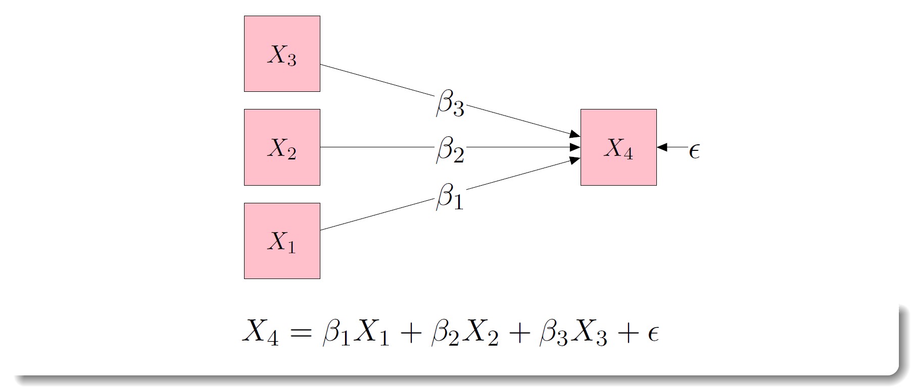
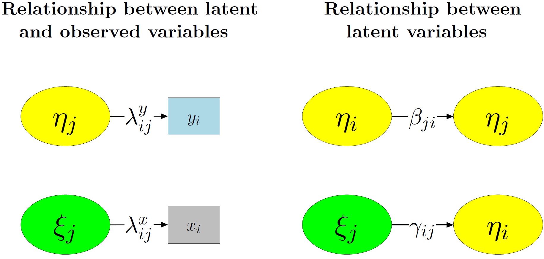
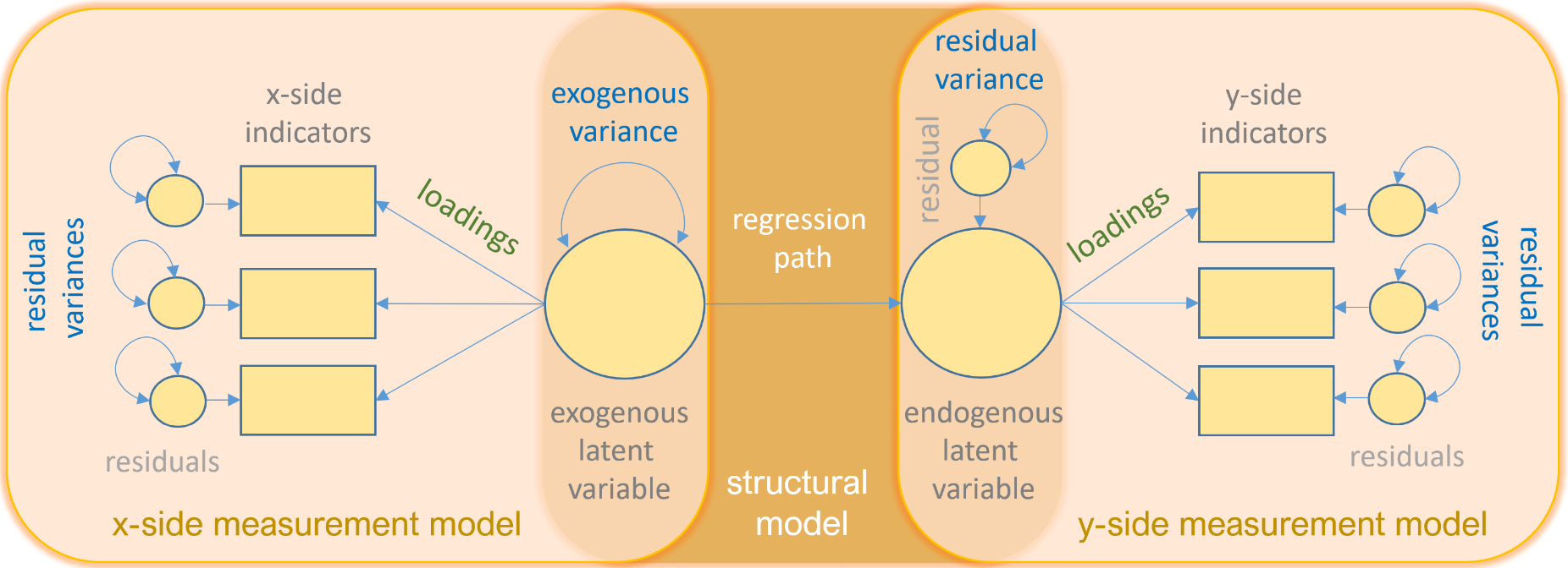
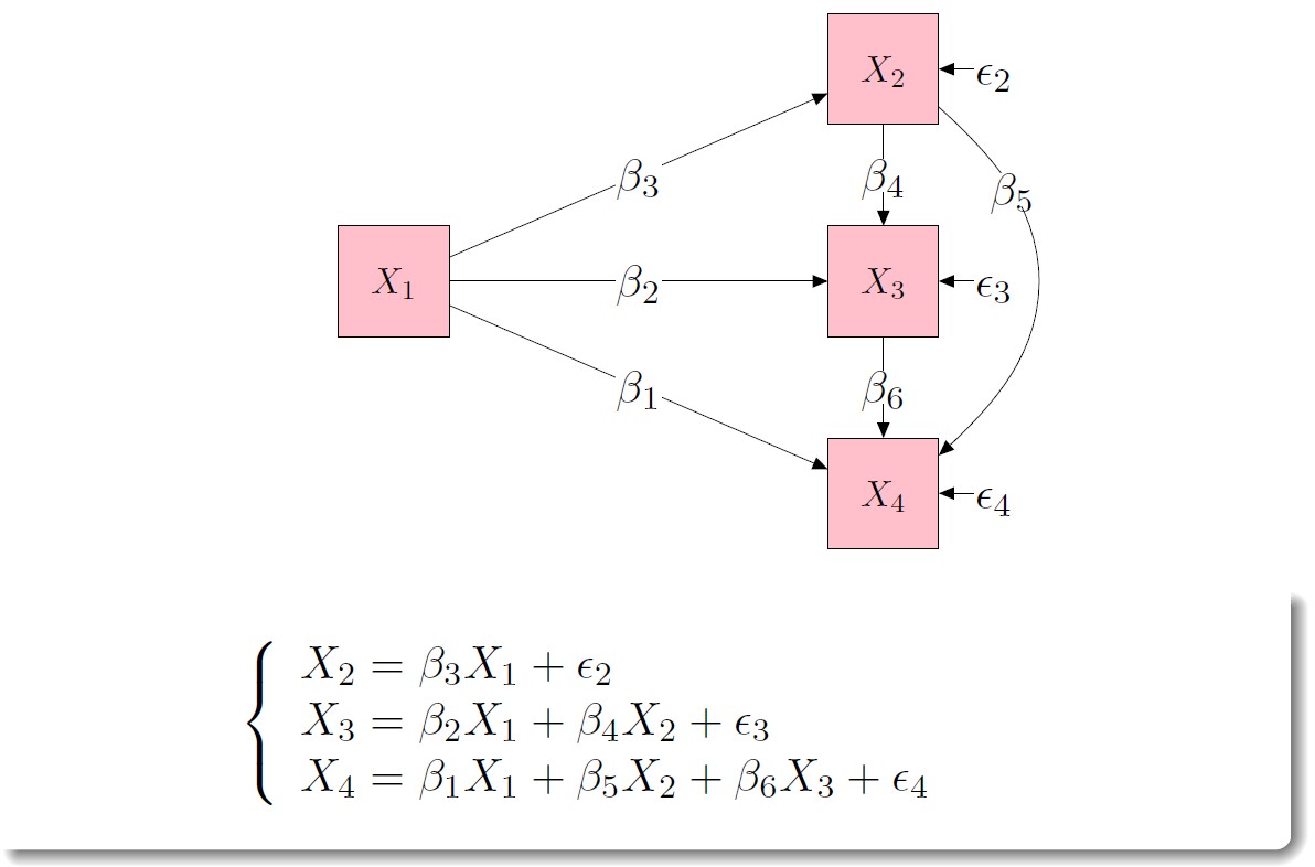
img credits to dr. Johnny Lin (youtube course)

Graphic relationships

A summary

SEM workflow

SEM steps (the workflow)

1. Model specification (theory → diagram → equations)
2. Model identification (can we estimate the parameters?)
3. Parameter estimation (choose estimator, get estimated matrices)
4. Model evaluation (global + local diagnostics)
5. Model modification / reporting (disciplined, transparent)

1) Model specification

What is a model

• A model is a formal representation of a theory and is composed by a set of parameters that we will estimate.

What you must state explicitly:

• which variables are connected (and in what direction)
• which errors/covariances are allowed
• which parameters are fixed, free, or constrained

2) Model identification

Basically, we want to know if there is enough information to identify a solution (aka estimate all the unknown parameters).

A model can be:

• Under-identified: there are MORE parameters to be estimated than elements in the covariance matrix (e.g., \(X + Y = 10\))

• Just-identified: the number of parameters to be estimated equals the number of elements in the covariance matrix (\(df = 0\))

• Over-identified: there are LESS parameters to be estimated than elements in the covariance matrix (\(df > 0\))

2) Model identification (intuition)

To ensure that the number of unknown parameters (\(t\)) is not greater than the number of nonredundant elements in the covariance matrix of \(q\) observed variables.

\[ t \leq \frac{q(q+1)}{2} \]

If the model is not identified, nothing else matters (no fit, no estimates).

Just-identified

Under-identified

Over-identified

3) Parameter estimation (what software does)

To estimate the model parameters we can use different estimation methods. These aim to estimate the model implied (theoretical) correlation matrix \(\boldsymbol{\Sigma}\), which is a function of the model parameters, and should hopefully be similar to the observed correlation matrix \(\boldsymbol{S}\).

Some of the many estimation methods are:

• Maximum Likelihood (ML), default in lavaan

• Unweighted Least Squares (ULS)

• Generalized Least Squares (GLS)

• Weighted Least Squares, Mean- and Variance-adjusted (WLSMV), default for ordinal variables in lavaan

• Diagonally Weighted Least Squares (DWLS)

4) Model evaluation

Is the model adequate? Do our parameter generate a theoretical matrix (\(\boldsymbol{\Sigma}\)) which is close to the empirical covariance matrix \(\boldsymbol{S}\)?

• Global fit: is the overall model plausible?
• Local fit: where does the model misfit?

We’ll do this properly in deck 03. Today: just remember that fit ≠ truth.

Formally:

\[ H_0 : \boldsymbol{\hat{\Sigma}}(\theta) = \boldsymbol{\Sigma} \]

where \(\boldsymbol{\Sigma}\) is the true covariance matrix among model variables, \(\theta\) the parameters vector, and \(\boldsymbol{\hat{\Sigma}}\) the reproduced covariance matrix.

5) Model modification (disciplined respecification)

At this point you are ‘free’ to modify the model based on the results obtained…AND THE THEORY!

• modifications are hypotheses
• modifications must be explicitly reported: both what you changed and why
• avoid overfitting (change only what is strictly needed/justified)

SEM world

Univariate regressions

Multivariate regressions

Path analysis

Confirmatory factor analysis (CFA)

SEM path analysis

t test with latent variables

Cross-lagged panel models

Growth curve models

And much more

THERE IS EVEN A JOURNAL ONLY FOR SEM

Structural Equation Modeling: A Multidisciplinary Journal

lavaan

lavaan (latent variable analysis) is actually THE package for SEM. You can use it to estimate a wide family of latent variable models, including: factor analysis, structural equation, longitudinal, multilevel, latent class, item respons, and missing data models…

..But also simple regressions

Bridge: from diagrams to lavaan

lavaan is mostly a model syntax language:

• you write relations like “y ~ x”
• lavaan estimates the parameters
• you read estimates + standard errors + fit indices + diagnostics

Think: “diagram ↔︎ equations ↔︎ lavaan syntax” (three representations of the same model).

Regression models

What you did since the beginning of the year (with link functions or not) was something like this \[ y = X\beta + \epsilon \] Where \(y\) is the response variable, \(X\) the set of predictors and \(\epsilon\) the error term.

These models,

• assume that all variables are directly observed/manifest
• allow measurement errors only in endogenous variables
• are just particular cases of SEM

SEM formula

In fact, the structural model of a SEM (i.e., excluding latent variables) is:

\[ Y = X^\ast B' + \zeta \]

Where

• \(Y\) is the (n x p) matrix of endogenous variables
• \(X^\ast\) is the n x (p + q) matrix of endogenous and exogenous variables
• \(B\) is the (p + q) x (p + q) coefficient matrices
• \(\zeta\) is the (p x q) matrix of errors in the equations

This looks pretty similar to the regression formula, but with some matrices! Univariate regression models are just a special case of this formula where the parameter matrix is full of 0

Regressions in matrices

   y x1 x2 x3
y  0  1  2  3
x1 0  0  0  0
x2 0  0  0  0
x3 0  0  0  0

   y x3 x2 x1
y  0  3  2  1
x3 0  0  5  4
x2 0  0  0  6
x1 0  0  0  0

From lm() to lavaan::sem()

A regression in base R:

fit_lm <- lm(y ~ x1 + x2, data = dat)
summary(fit_lm)

The same idea in lavaan :

library(lavaan)

mod <- '
  y ~ x1 + x2
'

fit <- sem(mod, data = dat)
summary(fit, standardized = TRUE)

A first example with simulated data

Imagine you want to predict scores in the test we will do at the end of this corse (\(y\)), based on your prior statistical knowledge (\(x_1\)) and interest (\(x_2\)):

First define the model

Second simulate the data

# Simulate knowledge and interest 
# as predictors of Y
set.seed(12)
N = 100
x1 = rnorm(N)
x2 = rnorm(N)
y = .35*x1 + .20*x2 + rnorm(N)
d <- data.frame(x1,x2,y)

cor(d)

      x1    x2    y
x1 1.000 0.016 0.39
x2 0.016 1.000 0.12
y  0.386 0.118 1.00

cov(d)

      x1    x2    y
x1 0.748 0.014 0.36
x2 0.014 0.998 0.13
y  0.364 0.129 1.19

lm regression

# fit a regression model
m <- lm(y ~ x1 + x2, data = d)
summary(m)

Call:
lm(formula = y ~ x1 + x2, data = d)

Residuals:
    Min      1Q  Median      3Q     Max 
-2.8022 -0.6244 -0.0259  0.7150  1.8090 

Coefficients:
            Estimate Std. Error t value Pr(>|t|)    
(Intercept)  -0.0251     0.1009   -0.25     0.80    
x1            0.4846     0.1172    4.14  7.5e-05 ***
x2            0.1226     0.1015    1.21     0.23    
---
Signif. codes:  0 '***' 0.001 '**' 0.01 '*' 0.05 '.' 0.1 ' ' 1

Residual standard error: 1 on 97 degrees of freedom
Multiple R-squared:  0.162, Adjusted R-squared:  0.145 
F-statistic: 9.36 on 2 and 97 DF,  p-value: 0.000191

Model fit and info

library(lavaan)
ml <- "y ~ 1 + x1 + x2" #1 + gives the intercept
fit <- sem(ml, data = d)
# summary(fit, rsquare=T)

lavaan 0.6-19 ended normally after 1 iteration

  Estimator                                         ML
  Optimization method                           NLMINB
  Number of model parameters                         4

  Number of observations                           100

Model Test User Model:
                                                      
  Test statistic                                 0.000
  Degrees of freedom                                 0

Parameter Estimates:

  Standard errors                             Standard
  Information                                 Expected
  Information saturated (h1) model          Structured

[...]

Model parameters

[...]
Regressions:
                   Estimate  Std.Err  z-value  P(>|z|)
  y ~                                                 
    x1                0.485    0.115    4.199    0.000
    x2                0.123    0.100    1.227    0.220

Intercepts:
                   Estimate  Std.Err  z-value  P(>|z|)
   .y                -0.025    0.099   -0.253    0.800

Variances:
                   Estimate  Std.Err  z-value  P(>|z|)
   .y                 0.987    0.140    7.071    0.000

R-Square:
                   Estimate
    y                 0.162

[...]

QUESTIONS? COMMENTS? What about lm?

Model plot

# And we can plot it
library(semPlot)
semPaths(fit, whatLabels = "parameters",
         edge.label.cex = 1.5, rotation = 2,
         residuals = F, sizeMan = 10, curve = 1.9,
         edge.color="black", edge.label.color="black")

Model matrices

We can also look at the matrices to enter in the SEM mindset

#The parameters matrix
inspect(fit)$beta

   y x1 x2
y  0  2  3
x1 0  0  0
x2 0  0  0

inspect(fit, "estimates")$beta

   y   x1   x2
y  0 0.48 0.12
x1 0 0.00 0.00
x2 0 0.00 0.00

#The residual var-covar matrix
inspect(fit)$psi

   y x1 x2
y  4      
x1 0  0   
x2 0  0  0

inspect(fit, "estimates")$psi

       y    x1    x2
y  0.987            
x1 0.000 0.741      
x2 0.000 0.014 0.988

Basic lavaan syntax

As you can see, the regression syntax of lavaan is actually the same as lm, but there is much more in lavaan.

Model specification sintax:

Syntax	Function	Example
~	Regress onto	Regress B onto A: B ~ A
~~	Residual (co)variance	Variance of A: A ~~ A Variance of A and B: A ~~ B
=~	Define a reflective LV	F1 is defined by items 1-4: F1 =~ i1 + i2 + i3 + i4
<~	Define a formative LV	F1 is defined by items 1-4: F1 <~ i1 + i2 + i3 + i4
:=	Define non-model parameters	u2 := x + y
*	Label or fix parameter	Z ~ b*X labels the regression as b

Basic lavaan functions

Function	Command
sem() / cfa()	Fit the SEM model (cfa is nested in sem…which is nested in lavaan)
fitMeasures()	Return fit indices of the SEM model
inspect()	Inspect/extract information that is stored in a fitted model
lavPredict()	Compute estimated latent scores
lavTestLRT()	Compare (nested) lavaan models
modificationIndices()	Compute the modification indices of a model
parameterEstimates()	Parameter estimates of a latent variable model
parameterTable()	Show the table of the parameters of a fitted model
standardizedSolution()	Show the table of the standardized parameters
simulateData()	Simulate data starting from a lavaan model syntax

Exercises (Lab 01)

Go to:

• labs/lab01_lavaan-basics.qmd (link)

You’ll practice:

• writing tiny models (~, ~~, =~)
• fitting with sem() / cfa()
• extracting key output (estimates, standardized, basic fit)

Take-home: 3 things

1. SEM is a language: diagrams, equations, syntax
   
2. SEM is a workflow: Specify → Identify → Estimate → Evaluate → Revise/Report
   
3. lavaan is your translator from theory → estimable model

Further reading / self-study

• Revisit the glossary in the repo as new terms appear
• Follow the course by Johnny Lin (youtube course)
• Follow Psicostat handZone meetings

Acknowledgments

Thanks to Massimiliano Pastore for his slides!