Path analysis & mediation

Observed-variable SEM (no latent variables yet)

Tommaso Feraco

Today in the workflow

Specify → Identify → Estimate → Evaluate → Revise/Report

Today: observed-variable path models and mediation (direct, indirect, total effects) + equivalence/pitfalls.
Next (03): model fit & diagnostics (global vs local, residuals, MI, disciplined respecification).

Learning objectives

By the end of this session you should be able to:

• Write a path model as a system of regressions
• Define direct, indirect, and total effects (and compute them in lavaan)
• Explain why indirect effects have non-normal sampling distributions
• Recognize just-identified path models (why “fit” can be uninformative)
• Explain (and fear, a little) model equivalence and causal interpretation limits

Path analysis

A path model is a set of linear regressions estimated jointly, with an explicit covariance structure and with at least one variable working as mediator.

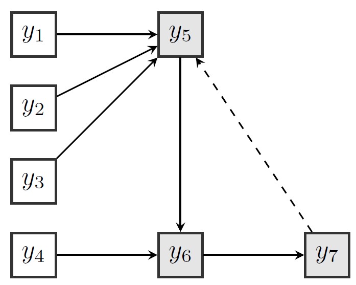
As usual, depicting the models is always the best way to understand our models.

Actually, this looks like a full SEM. Why? And why it isn’t, given the way latent variables should be represented?.

From “effects” to equations

A path diagram is shorthand for a system like:

\[ \begin{aligned} M &= i_M + aX + \varepsilon_M\\ Y &= i_Y + c'X + bM + \varepsilon_Y \end{aligned} \]

• \((X)\) exogenous (predictor)
• \((M\)) mediator (endogenous)
• \((Y)\) outcome (endogenous)

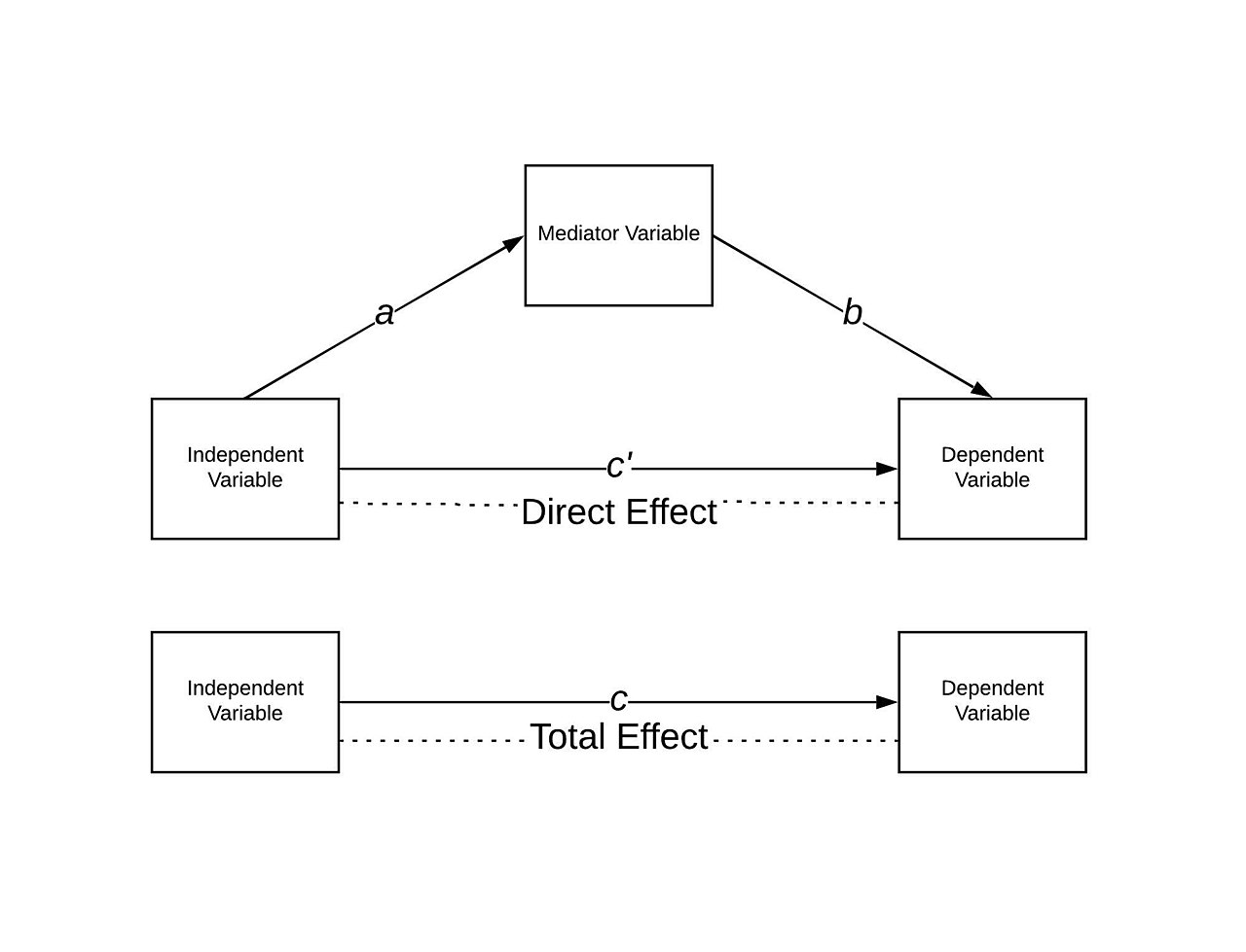
Mediation: three effects

\[ \text{Indirect} = ab \qquad \text{Direct} = c' \qquad \text{Total} = c = c' + ab \]

Interpretation (linear, continuous case):

• \((a)\): expected change in \((M)\) per unit change in \((X)\)
• \((b)\): expected change in \((Y)\) per unit change in \((M)\) (holding \((X)\) fixed)
• \((c')\): remaining effect of \((X)\) on \((Y)\) after \((M)\)

Diagram: mediation template

“Indirect effect” is not automatically “causal mediation”. Causal language requires assumptions!

Why SEM for mediation?

SEM makes it easy to:

• estimate the system jointly (including residual covariance if justified)
• compute functions of parameters (e.g., \((ab)\), totals, contrasts)
• add covariates, multiple mediators, constraints, and (later) measurement models

Indirect effects are just products

The indirect effect is a product \((ab)\). Even if \((\hat a)\) and \((\hat b)\) are approximately normal, the product is not.

A common large-sample approximation (delta method):

\[ \mathrm{Var}(\widehat{ab}) \approx b^2\mathrm{Var}(\hat a) + a^2\mathrm{Var}(\hat b) + 2ab\,\mathrm{Cov}(\hat a,\hat b) \]

Sobel test (same idea, historically popular):

\[ z = \frac{\widehat{ab}}{\sqrt{\widehat{\mathrm{Var}}(\widehat{ab})}} \]

In practice, bootstrap is often preferred for indirect effects (especially with small–moderate \(N\)).

lavaan: mediation as a model + defined parameters

You already know ~ and ~~. The new piece is:

• labels (a*X) and defined parameters (ind := a*b)

library(lavaan)

mod_med <- '
  # structural regressions
  M ~ a*X
  Y ~ cprime*X + b*M

  # (optional) exogenous variance
  X ~~ X

  # defined effects
  ind := a*b
  tot := cprime + (a*b)
'

fit <- sem(mod_med, data = dat, meanstructure = TRUE)
summary(fit, standardized = TRUE)

Note

in lavaan * is not an interaction term but an assignment/lableing

Bootstrap the indirect effect

fit_b <- sem(
  mod_med, data = dat,
  se = "bootstrap", bootstrap = 2000,
  meanstructure = TRUE
)

parameterEstimates(fit_b, ci = TRUE, level = .95,
                   standardized = TRUE) |>
  subset(op %in% c("~", ":="))

Interpretation:

• focus on \((ab)\) estimate and its CI
• bootstrap CI is not magic; it’s still conditional on model assumptions

A richer example: multiple indirect paths

Sometimes the theory implies more than one mediated route.

(Example structure; your variables will differ.)

Notation. If there are two indirect paths:

\[ \text{ind}_1 = a_1 b_1, \qquad \text{ind}_2 = a_2 b_2, \qquad \text{total indirect} = \text{ind}_1 + \text{ind}_2 \]

You can define each and test/CI them separately.

lavaan: multiple indirect effects (template)

mod_multi <- '
  # example: two mediators in parallel
  M1 ~ a1*X
  M2 ~ a2*X
  Y  ~ cprime*X + b1*M1 + b2*M2

  # optional: allow mediators to covary
  M1 ~~ M2

  ind1 := a1*b1
  ind2 := a2*b2
  indT := ind1 + ind2
  tot  := cprime + indT
'

fit <- sem(mod_multi, data = dat, se = "bootstrap", bootstrap = 2000)
summary(fit, standardized = TRUE)

Parallel mediators are easy to write; the hard part is interpretation (confounding, causal ordering, measurement).

Standardized vs unstandardized effects

• Unstandardized (\(\hat a\), \(\hat b\), \(\widehat{ab}\)) are in original units → best for substantive interpretation if units matter.
• Standardized effects help compare across variables/scales.

For a simple mediation (continuous variables), a fully standardized indirect effect is:

\[ (ab)_{\text{std}} = ab \cdot \frac{\sigma_X}{\sigma_Y} \]

(because the (\(\sigma_M\)) cancels)…but lavaan does it for you.

Identification + “fit can be perfect”

Many basic path/mediation models are just-identified:

• no degrees of freedom \((df = 0)\)
• the model reproduces the sample covariance matrix exactly
• fit indices will look “perfect” even if the causal story is wrong

A useful counting rule:

\[ df = \frac{p(p+1)}{2} - t \]

where \((p)\) = observed variables, \((t)\) = free parameters.

When can mediation be interpreted causally?

At minimum, you need assumptions such as:

• temporal ordering (X precedes M precedes Y)
• no unmeasured confounding for:
  • \((X \rightarrow M)\)
  • \((M \rightarrow Y)\)
  • \((X \rightarrow Y)\)
• correct model form (linearity, additivity, no omitted interactions unless modeled)
• very strong theoretical assumptions

Tip

For deep dives into causality (and many other things), follow Julia Rohrer and the100CI blog.

Diagnostics (what to check now)

Even before learning “fit”, you should check:

• sign and magnitude of parameters (are they plausible?)
• standard errors / CIs (especially for \(ab\))
• residual variances (negative? huge? suspiciously tiny?)
• collinearity among predictors/mediators (unstable estimates)

For mediation, your first diagnostic is often conceptual: is this ordering defensible? then statistical: is \((ab)\) estimated precisely?

Can ‘sex’ be a mediator?!

Exercises (Lab 02)

Go to:

• labs/lab02_path-mediation.qmd link

You will practice:

1. Fit a simple mediation with bootstrap CI for \((ab)\)
2. Add covariates (and observe what happens to \((a)\), \((b)\), and \((c')\))
3. Compare partial vs “full” mediation (constraint \((c'=0)\))
4. Fit a parallel-mediator model and interpret \((ind_1)\), \((ind_2)\), \((ind_T)\)

Pitfall callout: “full mediation” is rarely a good goal

Even if \((c')\) is small/non-significant:

• it does not prove the direct path is zero
• power and measurement error can make \((c')\) hard to detect
• the direct effect can be suppressed or masked by omitted paths

Better framing:

• focus on effect sizes + uncertainty
• test theoretically motivated constraints (and report them transparently)

Take-home: 3 things

1. Mediation effects are functions of parameters (\((ab)\), \((c'+ab)\)) → compute them explicitly
   
2. The indirect effect’s sampling distribution is non-normal → bootstrap is often sensible
   
3. Path models are vulnerable to equivalence → fit alone cannot justify causal stories

Further reading / self-study

Some blogposts you may like

• Reviewer notes: That’s a very nice mediation analysis you have there. It would be a shame if something happened to it.
• Causal Inference | Hypothesis Testing | All at Once
• Longitudinal data don’t magically solve causal inference

A paper, still Rohrer (2022): That’s a Lot to Process! Pitfalls of Popular Path Models link

References

Rohrer, J. M., Hünermund, P., Arslan, R. C., & Elson, M. (2022). That’s a Lot to Process! Pitfalls of Popular Path Models. Advances in Methods and Practices in Psychological Science, 5(2), 25152459221095827. https://doi.org/10.1177/25152459221095827