CFA: measurement models, identification, reliability

From items to constructs (measurement-first)

Tommaso Feraco

Today in the workflow

Specify → Identify → Estimate → Evaluate → Revise/Report

Today: the measurement part — CFA (and reliability from CFA).
Two-step mindset: measure first, then relate constructs (SEM deck 05).

Learning objectives

By the end of this session you should be able to:

• Explain the difference between EFA and CFA
• Write the CFA measurement model in equations and matrices
• Understand identification & scaling (marker vs std.lv)
• Fit CFA models in lavaan and interpret loadings, factor correlations, and residual variances
• Use local diagnostics in CFA (residuals, MI/EPC) without “fit hacking”
• Compute and report reliability from CFA (ω-family; and (briefly) bifactor implications)

Outline

• Factor analysis: what problem are we solving?
• EFA vs CFA (confirmatory stance)
• CFA model: equations, matrices, implied covariance
• Identification and constraints (scaling + rules)
• CFA in R (lavaan) + interpretation
• Reliability from CFA
• Bifactor model

Factor analysis

Important

Factor analysis models believe that a small number of latent dimensions explain systematic covariance among many observed variables.

Warning

PCA is not a factor analysis. It does not assume the ‘existence’ of any latent trait.

Exploratory Factor Analysis (EFA)

EFA: discover a plausible loading pattern.

• loadings are “free” (rotation chooses a representation)
• useful for exploration and item development
• weak theory → eavily exploratory

Confirmatory Factor Analysis (CFA)

CFA: test a specific measurement hypothesis.

• you specify which loadings are zero vs free
• you can impose constraints (equal loadings, orthogonality, hierarchies)
• fit and diagnostics evaluate a theoretically constrained model

CFA is not a fancy EFA: it is a confirmatory claim with theoretical assumptions and meanings.

General formula

The general CFA model can be written as:

\[ \begin{aligned} \mathbf{x} &= \mathbf{\Lambda}_x\,\mathbf{\xi} + \mathbf{\delta} \\ \mathbf{y} &= \mathbf{\Lambda}_y\,\mathbf{\eta} + \mathbf{\epsilon} \end{aligned} \]

where \((\mathbf{x})\) and \((\mathbf{y})\) are observed variables, \((\mathbf{\xi})\) and \((\mathbf{\eta})\) are latent factors, and \((\mathbf{\delta})\) and \((\mathbf{\epsilon})\) are errors of measurement.

The general formula explained (scalar form)

\[ \begin{aligned} y &= b_0 + b_1 x + \epsilon \\ y_1 &= \tau_1 + \lambda_1\eta + \epsilon_1 \end{aligned} \]

\[ \begin{bmatrix} y_1 \\ y_2 \\ y_3 \end{bmatrix} = \begin{bmatrix} \tau_1 \\ \tau_2 \\ \tau_3 \end{bmatrix} + \begin{bmatrix} \lambda_1 \\ \lambda_2 \\ \lambda_3 \end{bmatrix} (\eta_1) + \begin{bmatrix} \epsilon_1 \\ \epsilon_2 \\ \epsilon_3 \end{bmatrix} \]

Measurement-first implications (reflective realism)

When we draw \((\mathbf{\Lambda})\) (\((\Rightarrow)\)) from latent to observed, we assume reflective latent variables:

• ARROWS are ARROWS: the construct affects responses
• “realist” interpretation: the latent variable is something that exists (at least as a stable attribute)
• observed scores = construct signal + measurement error

Pragmatic “just a summary” interpretations are not neutral: they imply different measurement models (PCA/EGA/…).

Important

Asserting that a latent variable ‘exists’ does not imply that there is one and only one entity/factor explaining the observations. A multitude, even millions, of factors (e.g., genes, ses, environment, health) can form the latent variable

The implied covariance (the single most important equation)

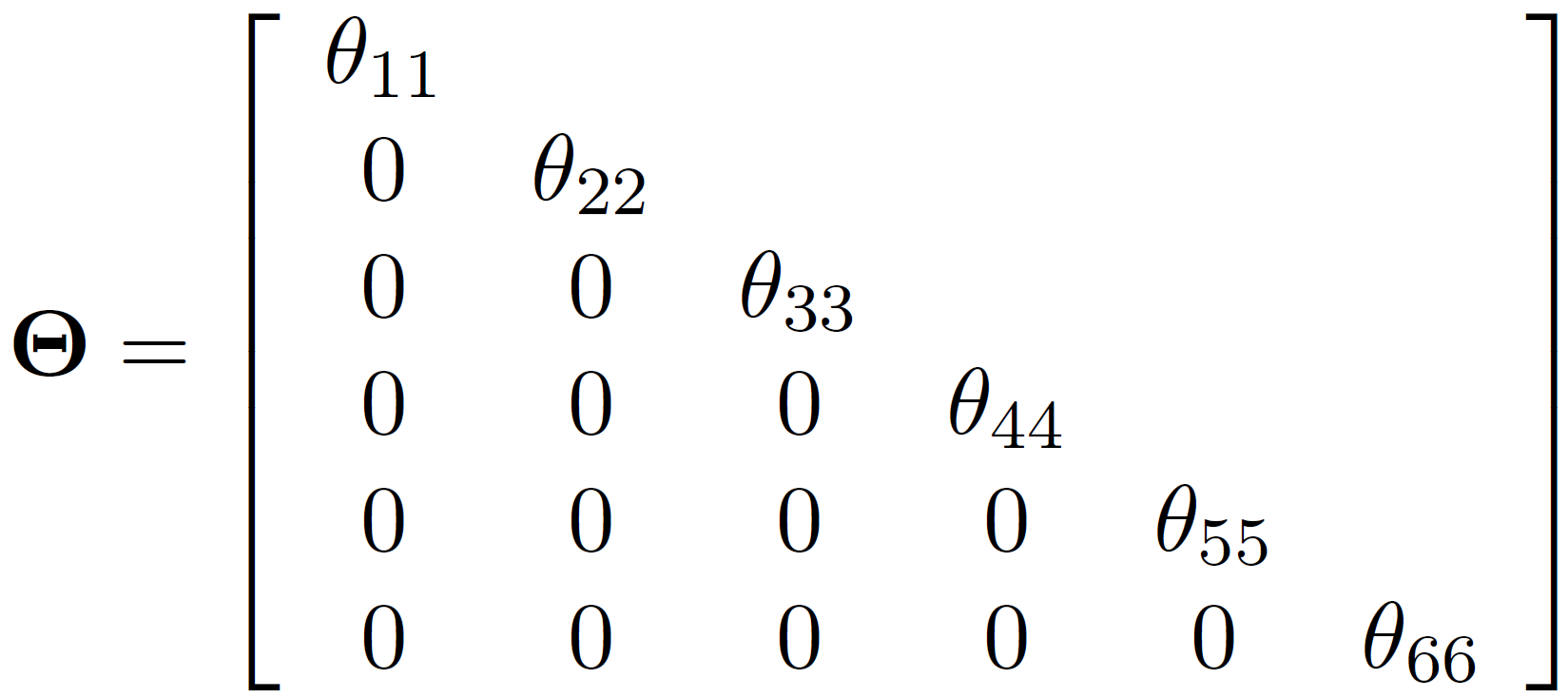
For a standard CFA with latent covariance \((\Phi)\) and residual covariance \((\Theta)\):

\[ \Sigma = \Lambda \Phi \Lambda' + \Theta \]

This is why:

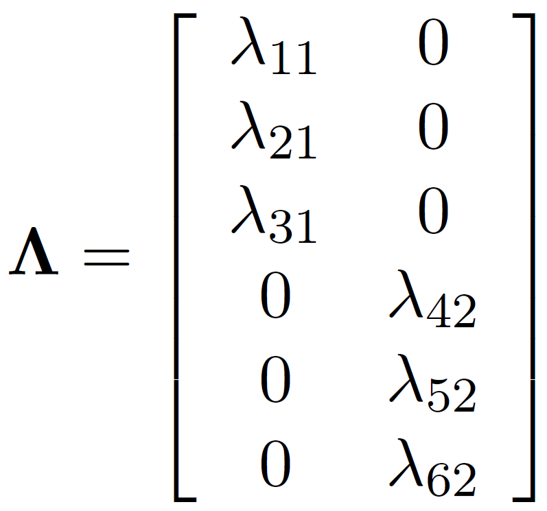
• loadings \((\Lambda)\) and factor correlations \((\Phi)\) jointly shape observed covariances
• correlated residuals (off-diagonal \((\Theta)\)) are extra covariance not explained by factors

Lambda: matrix of loadings

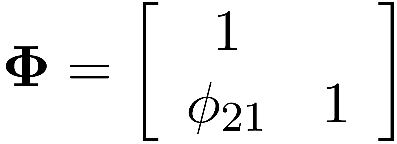
Phi: latent variance-covariance matrix

Theta: residual variance-covariance matrix

CFA models

CFA “model families”

Key design choices:

• one factor vs multiple factors
• are factors correlated?
• orthogonal vs oblique
• hierarchical / second-order?
• bifactor structure?

All have statistical and theoretical consequences.

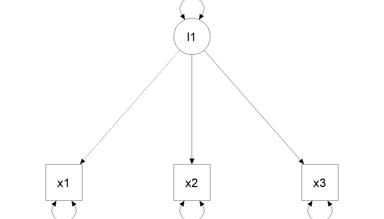
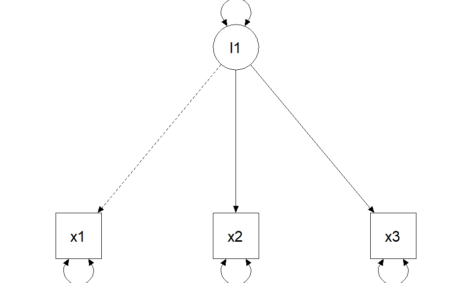
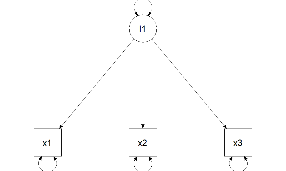
One-factor model

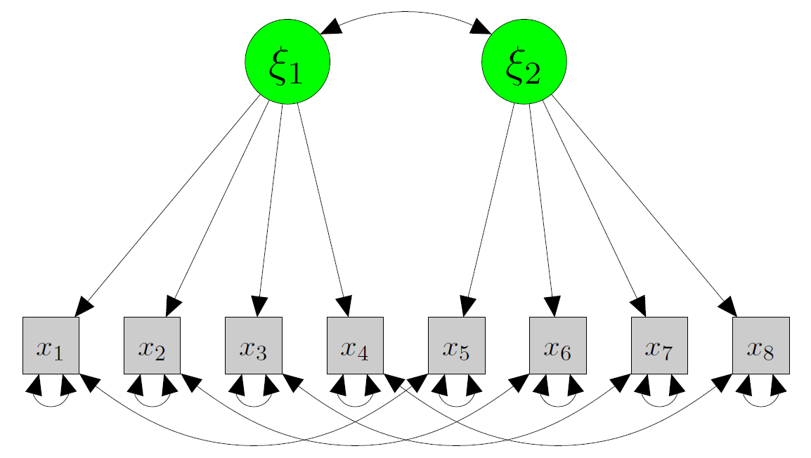
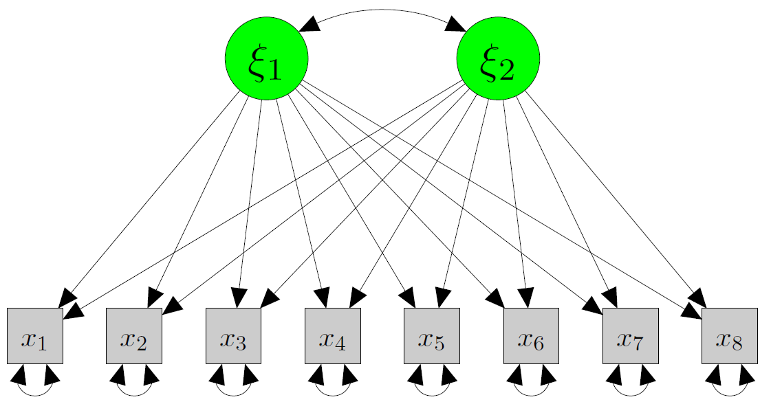
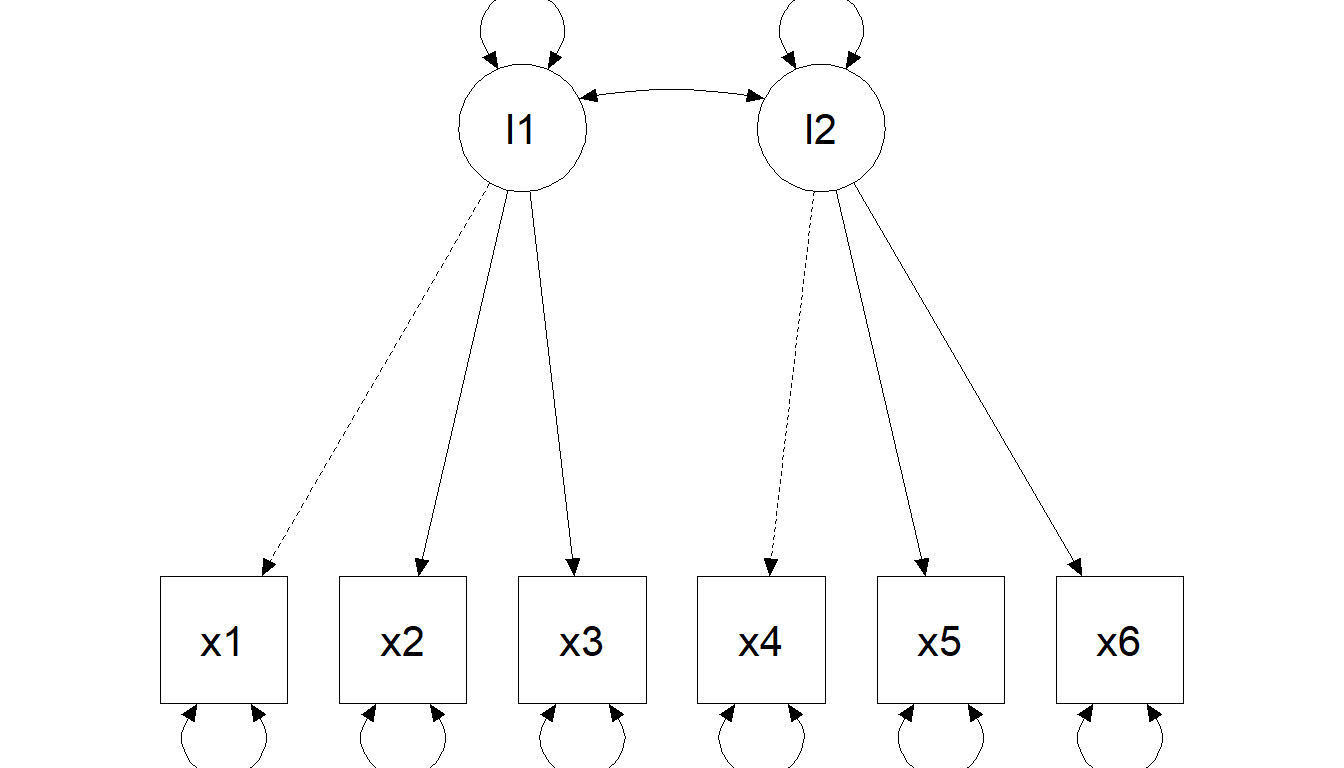
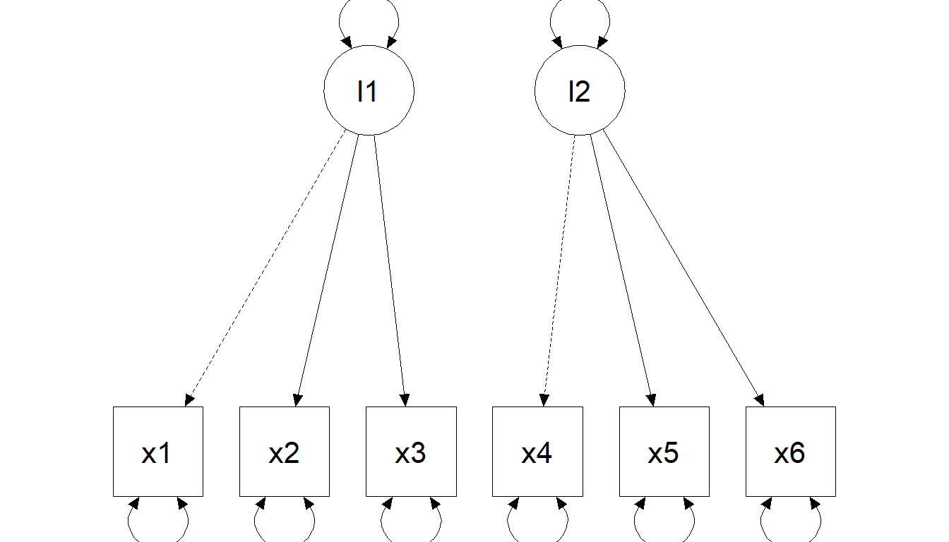
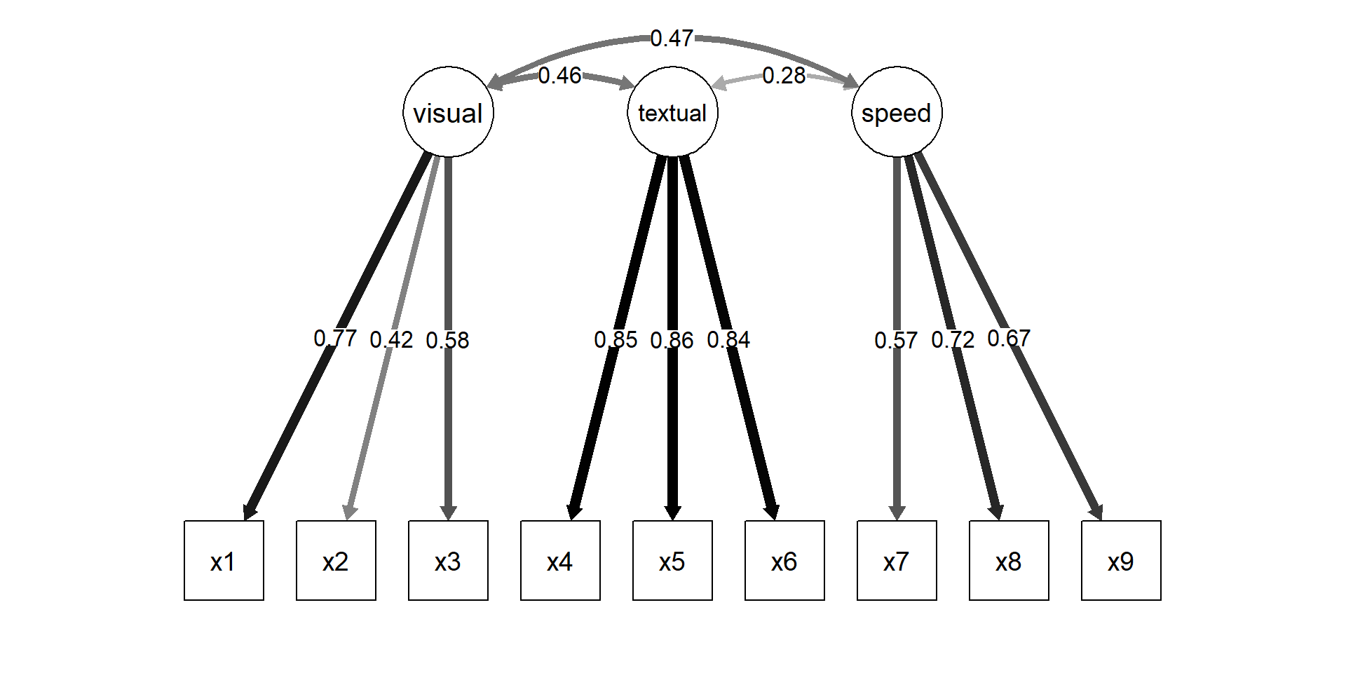
Two-factor model (correlated factors)

Two-factor model (orthogonal factors)

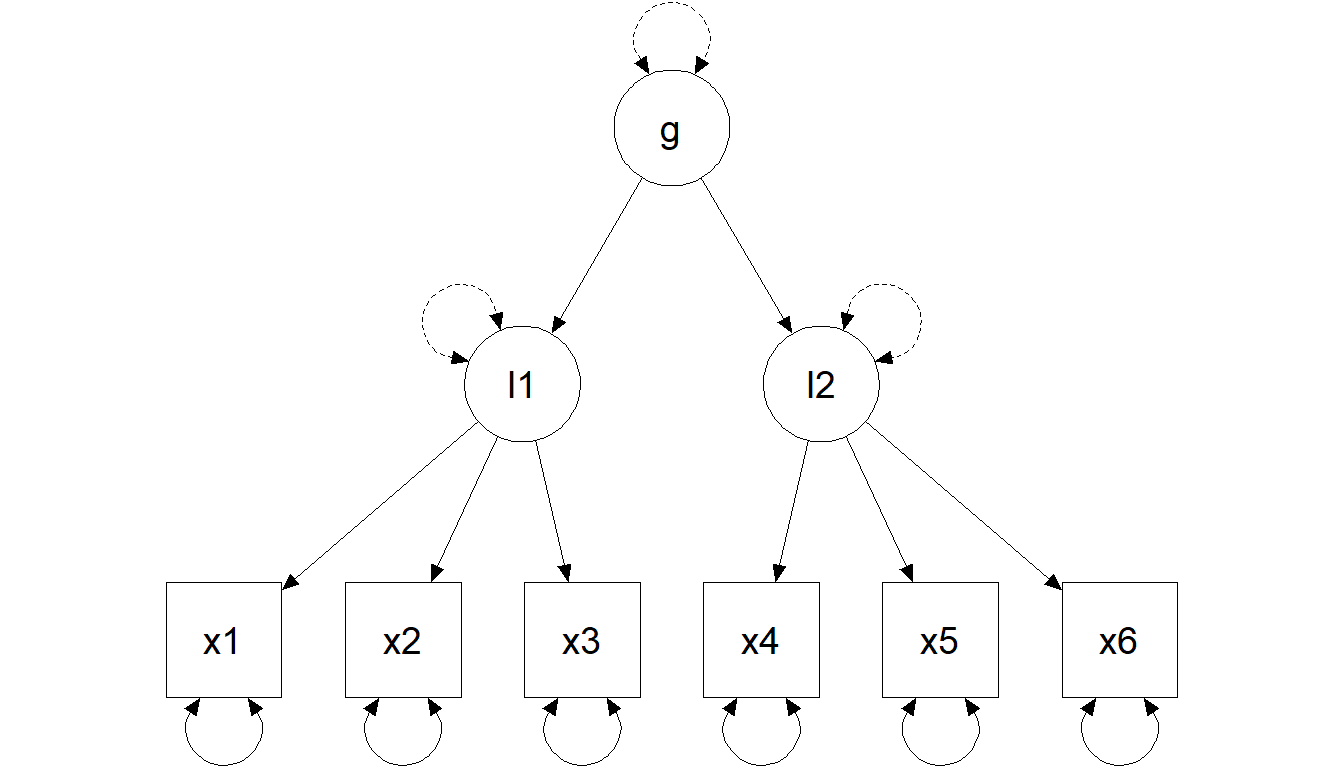
Hierarchical model (second-order factor)

R

In R (lavaan grammar for CFA)

Core operator:

• =~ defines a factor from its indicators

m <- '
  F1 =~ y1 + y2 + y3
  F2 =~ y4 + y5 + y6
  F1 ~~ F2          # factor covariance (oblique)
'

fit <- cfa(m, data = dat)  # or sem(m, data = dat)
summary(fit, standardized = TRUE, fit.measures = TRUE)

Constraints (scaling)

To estimate latent-variable models, you must scale each factor. Two common strategies:

• Standardize latent variables: fix factor means to 0 and factor variances to 1 (std.lv = TRUE).
• Marker method: set one loading (\((\lambda)\)) per factor to 1 (lavaan default).

fit <- cfa(m, data = dat, std.lv = TRUE) # Std latent variables
fit <- cfa(m, data = dat, std.lv = FALSE) # Marker method

Constraints explained (marker vs standardization)

\[ \Sigma = \Lambda\Phi\Lambda' + \Theta \]

Marker method (fix one loading to 1)

Standardization (fix factor variance to 1)

Note

Scaling changes the metric of unstandardized loadings, not the implied covariance model.

Identification & evaluation

Identification rules

For CFA, common identification rules include:

• the t-rule
• the Three-Indicator Rule
• the Two-Indicator Rule

The t-rule

Necessary but not sufficient:

\[ t \leq \frac{q(q+1)}{2} \]

where \((t)\) is the number of free parameters and \((q)\) the number of observed variables.

Intuition: the number of nonredundant elements in \((S)\) is the maximum number of “equations”; if unknowns exceed equations, identification is impossible.

The Three-Indicator Rule

A sufficient (not necessary) condition (with diagonal \((\Theta)\)):

1. One-factor model: at least three indicators with nonzero loadings.
2. Multifactor model is identified if:
   1. ≥ 3 indicators per factor
   2. each row of \((\Lambda)\) has one and only one nonzero element (simple structure)
   3. \((\Theta)\) is diagonal

The Two-Indicator Rule

A sufficient (not necessary) condition for models with >1 factor:

• \((\Theta)\) diagonal
• each factor scaled (one \((\lambda)\) fixed to 1, or std.lv=TRUE)
• plus:
  1. ≥ 2 indicators per factor
  2. each row of \((\Lambda)\): one nonzero element
  3. \((\Theta)\) diagonal
  4. each row of \((\Phi)\) has at least one nonzero off-diagonal element

CFA evaluation (see deck 03)

Global indices are the same as in deck 03 (χ², CFI/TLI, RMSEA+CI, SRMR).
What becomes CFA-specific is local misfit interpretation:

• big residual correlations → local dependence / method effects / cross-loadings
• MI/EPC candidates typically propose:
  • cross-loadings (theory-threatening)
  • correlated residuals (requires a clear justification)
  • factor covariances / (rarely) indicator-level regressions

Warning

Fit ≠ validity. “Improving fit” can destroy the meaning of a factor model if you add substantively implausible parameters.

A disciplined CFA respecification mindset

• First: check items (loadings, residual variances, signs)
• Then: check patterns (blocks of residual correlations)
• MI/EPC only after you have a hypothesis for the misfit
• Prefer fewer, theory-consistent modifications over many “small fixes”
• Report the respecification path transparently (what changed and why)

Holzinger & Swineford (1939)

dat <- HolzingerSwineford1939

m_hs <- '
  visual  =~ x1 + x2 + x3
  textual =~ x4 + x5 + x6
  speed   =~ x7 + x8 + x9
'
fit_hs <- cfa(m_hs, data = dat, std.lv = TRUE)

Interpret loadings and factor correlations

pe <- parameterEstimates(fit_hs, standardized = TRUE)
pe[pe$op %in% c("=~","~~") & pe$lhs %in% c("visual","textual","speed"),
   c("lhs","op","rhs","est","se","pvalue","std.all")]

       lhs op     rhs   est    se pvalue std.all
1   visual =~      x1 0.900 0.081      0   0.772
2   visual =~      x2 0.498 0.077      0   0.424
3   visual =~      x3 0.656 0.074      0   0.581
4  textual =~      x4 0.990 0.057      0   0.852
5  textual =~      x5 1.102 0.063      0   0.855
6  textual =~      x6 0.917 0.054      0   0.838
7    speed =~      x7 0.619 0.070      0   0.570
8    speed =~      x8 0.731 0.066      0   0.723
9    speed =~      x9 0.670 0.065      0   0.665
19  visual ~~  visual 1.000 0.000     NA   1.000
20 textual ~~ textual 1.000 0.000     NA   1.000
21   speed ~~   speed 1.000 0.000     NA   1.000
22  visual ~~ textual 0.459 0.064      0   0.459
23  visual ~~   speed 0.471 0.073      0   0.471
24 textual ~~   speed 0.283 0.069      0   0.283

Reliability from CFA (ω family)

reliability(fit_hs) # Deprecated :(

compRelSEM(fit_hs)

 visual textual   speed 
  0.612   0.885   0.686 

AVE(fit_hs)

 visual textual   speed 
  0.371   0.721   0.424 

We emphasize ω-family (omega) reliability because it aligns with the CFA model; α is a special (often unrealistic) case.

Graphical representation

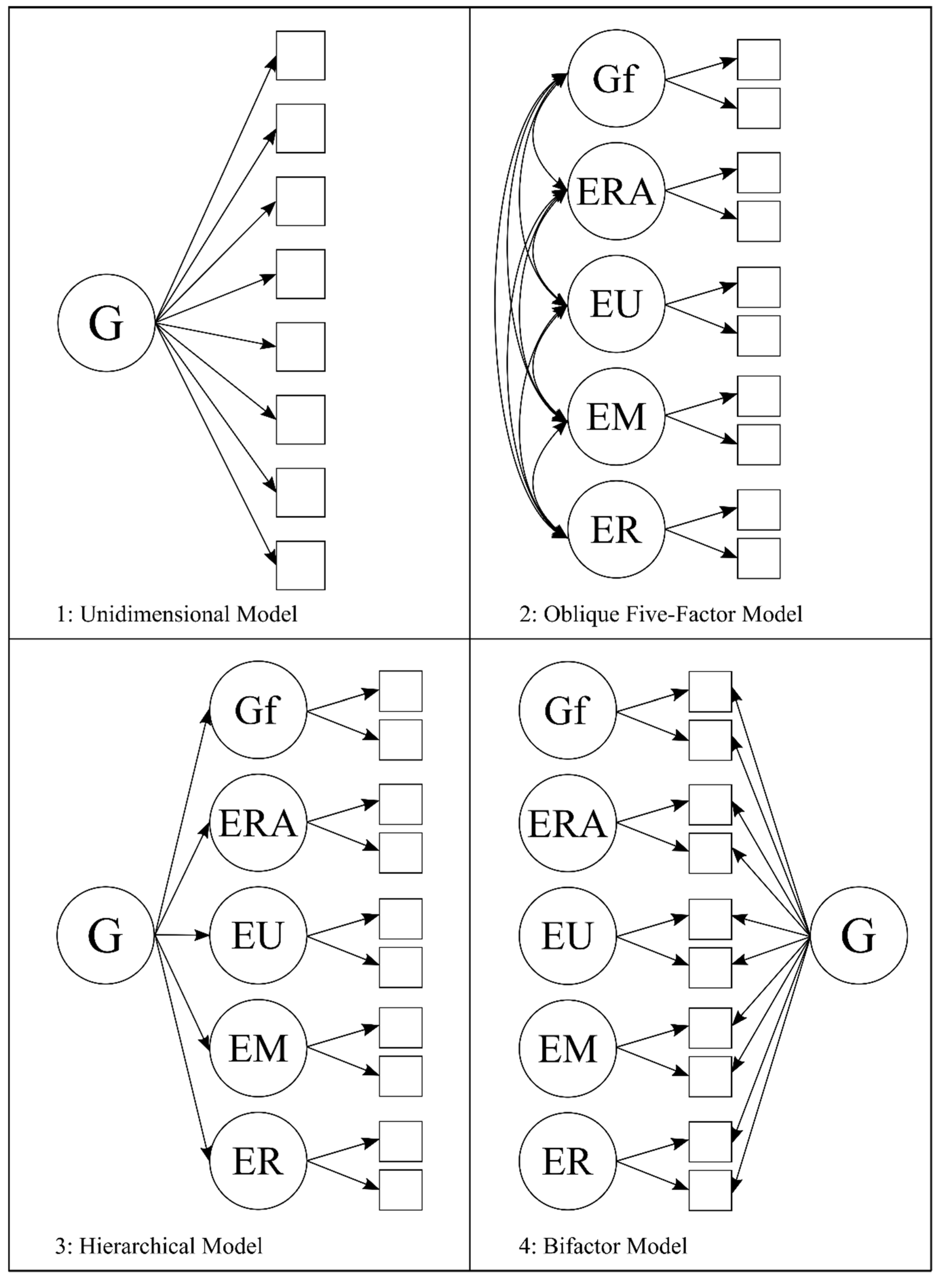
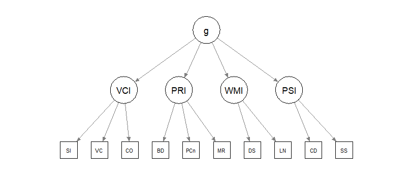
A hierarchical intelligence example

Theory: test scores are affected by specific abilities (e.g., processing speed) that are influenced by an overarching factor (\(g\)).

In practice, you should validate first-order abilities before jumping to a second-order model.

Second-order CFA (syntax template)

N = 1000
mg <- "
VCI =~ .60*SI + .60*VC + .60*CO
PRI =~ .60*BD + .60*PCn + .60*MR
WMI =~ .60*DS + .60*LN
PSI =~ .60*CD + .60*SS
g   =~ .70*VCI + .70*PRI + .70*WMI + .70*PSI
"
datg <- simulateData(mg, N)
S<-cov(datg)

m2 <- "
VCI =~ SI + VC + CO
PRI =~ BD + PCn + MR
WMI =~ DS + LN
PSI =~ CD + SS
g   =~ VCI + PRI + WMI + PSI # HERE IS THE SECOND-ORDER
"
fit2 <- sem(m2, std.lv = TRUE, sample.cov = S, sample.nobs = N)

Note

Note that we use sample.cov and sample.nobs arguments instead of data. In SEM you can fit the models from the covariance matrix and ‘ignore’ the raw data.

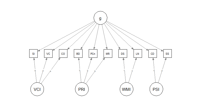
A second theoretical model: bifactor

Parallel theories: test scores are affected by a general factor (\(g\)) and by specific abilities that explain remaining variance.

All factors are set to be orthogonal.

Bifactor model in R

mb <- "
VCI =~ a*SI + a*VC + a*CO
PRI =~ b*BD + b*PCn + b*MR
WMI =~ c*DS + c*LN
PSI =~ d*CD + d*SS
g   =~ SI + VC + CO + BD + PCn + MR + DS + LN + CD + SS
"

fitb <- sem(
  mb,
  orthogonal = TRUE, #!!!!!!
  std.lv = TRUE,
  sample.cov = S,
  sample.nobs = N
)

Note

Note that loadings in bifactor models are often costrained to be equal within the same specific factors. This is done to ease convergence but should be justified and transparently reported.

Bifactor: interpretation requires diagnostics (not just fit)

Bifactor often improves fit by absorbing residual covariance.

fitmeasures(fitb, fit.measures = c("cfi","rmsea","srmr"))

  cfi rmsea  srmr 
0.985 0.026 0.025 

Before interpreting:

• is the general factor strong enough? (ECV / ωH / H)
• are specific factors meaningful or “junk factors”?
• do constraints (orthogonality, equal loadings) make sense?

A bifactor model that “fits” can still be a bad measurement story.

Bifactor diagnostics: is there a strong general factor?

library(BifactorIndicesCalculator)
bi <- bifactorIndices(fitb)

Model-level bifactor indices

Model	ECV.g	PUC	Omega.g	OmegaH.g
1	0.351	0.822	0.768	0.513

ECV.g = proportion of common variance explained by the general factor.

PUC = proportion of correlations uncontaminated by overlap among specific factors.

Omega.g = reliability of the observed total score.

OmegaH.g = proportion of total-score variance attributable uniquely to g.

Warning

Interpretation

These results do not support a strong general factor.

ECV.g = ~0.30: g explains only about 30% of common variance; OmegaH.g ~ 0.40: only about 40% of total-score variance is uniquely due to g. PUC ~ 0.80 is fairly high, but high PUC does not rescue weak ECV.g and OmegaH.g.

Are the specific factors interpretable beyond g?

Factor-level bifactor indices

	ECV_SS	ECV_GS	Omega	OmegaH	H	FD
VCI	0.656	0.344	0.666	0.438	0.516	0.699
PRI	0.705	0.295	0.664	0.472	0.541	0.720
WMI	0.614	0.386	0.575	0.353	0.398	0.627
PSI	0.580	0.420	0.511	0.296	0.332	0.573
g	0.351	0.351	0.768	0.513	0.614	0.727

ECV_SS = proportion of common variance in a factor’s own items due to that specific factor.

ECV_GS = proportion of common variance in those same items due to the general factor.

Omega = reliability of the observed factor score, counting all modeled common variance.

OmegaH = reliable variance attributable to the factor itself, net of the other factors.

H = construct replicability.

FD = factor determinacy, that is, how well factor scores are defined.

Note

Interpretation. For all four group factors, ECV_SS > ECV_GS: within each item cluster, the specific factor is stronger than g. But OmegaH, H, and FD are modest for both the group factors and g: none appears especially strong or highly replicable.

Overall, the structure looks multidimensional, not essentially unidimensional.

Item-level evidence: do any items mainly reflect g?

Item-level IECV values

	IECV
SI	0.367
VC	0.352
CO	0.309
BD	0.390
PCn	0.290
MR	0.191
DS	0.383
LN	0.388
CD	0.408
SS	0.432

IECV = proportion of an item’s common variance accounted for by the general factor. High IECV means the item behaves mostly like an indicator of g. Low IECV means the item retains substantial non-general variance.

Important

Interpretation

Here, IECV values range from about 0.17 to 0.40.

No item behaves mainly as an indicator of the general factor. The general factor is therefore not dominant at the item level. This reinforces the earlier conclusion: the bifactor model does not justify treating the scale as essentially unidimensional.

Exercises (Lab 04)

Go to:

• labs/lab04_cfa_reliability_omegas.qmd link

You will practice:

1. Fit and compare 1-factor vs correlated-factors CFA
2. Inspect local misfit (residual correlations + MI/EPC) with a theory filter
3. Compute reliability (ω) from CFA and report it
4. (Optional) Fit a bifactor model and evaluate interpretability (ωH / ECV)

Take-home: 3 things

1. CFA is a confirmatory measurement claim: zeros and constraints are theory
   
2. Identification/scaling is not a nuisance—it’s the metric of your construct
   
3. Reliability and validity are model-based: fit helps, but fit ≠ validity

Further reading / self-study

• Classic SEM measurement chapters (CFA fundamentals; see course website reading list)

• Maybe one day

  • extras/ex10_bifactor_esem_method-factors.qmd — bifactor/ESEM/method factors (advanced)
  • extras/ex05_miivs_factor-score-regression.qmd — factor scores & regression (later)

Acknowledgments

Thanks to Massimiliano Pastore for his slides!

References