SEM with ordinal variables

Ordinal indicators: thresholds, DWLS/WLSMV, and invariance

Tommaso Feraco

Today in the workflow

Specify → Identify → Estimate → Evaluate → Revise/Report

Today: extending SEM to ordinal (ordered-categorical) indicators:
thresholds, polychoric correlations, DWLS/WLSMV (and ULS), and what changes in model fit and invariance.

Learning objectives

By the end of this session you should be able to:

Explain the latent-response view of ordinal items and the role of thresholds
Know when treating Likert items as continuous is risky (few categories / skewed distributions)
Fit ordinal CFA/SEM in lavaan using ordered= and appropriate estimators (DWLS/WLSMV/ULS)
Understand how (and why) global fit indices behave differently with ordinal data
Run MG-CFA invariance with ordinal indicators (thresholds first, then loadings)

Introduction

In psychology we rarely have data that are normally distributed or that follow a continuous distribution. Our data are probably ordinal or the consequence of ordinal/dichotomous processes:

set.seed(42); n=10000; items = 30;
score <- rbinom(n,items, rnorm(n,.80,.10))

COMMENTS?

Introduction

However, we postulate that they are generated from continuous normal latent distributions

COMMENTS?

Likert scales

This also applies to Likert scales, where the difference between reporting a score of 1 or 2, and the difference between reporting a score of 2 or 3 is not the same!

The `adaptability` data

And in real data Likert items are NEVER normally distributed

Wrong correlations

Unfortunately, when we use data that follow discrete distributions and treat them as they were continuous, we can fail to recreate true correlation matrices accurately. That’s why you usually use polychoric correlations with dichotomous or ordinal variables.

This, of course, has consequences on SEM parameters, which are based on covariance

Data were generated from a multivariate normal distribution using MASS::mvrnorm and then manually truncated on a 3-point scale

In `lavaan` and SEM

To estimate a model treating items/observations as ordinal data, we need to change the estimationd method

ML is not always accurate with ordinal data (especially with few categories)
lavaan, when ordered is TRUE, automatically use WLSMV (Weighted Least Squares Means and Variance-adjusted)
A great alternative is ULS, but has more convergence problems
We can also use robust ML alternatives, like MLR
Other available estimators: lavaan tutorial on estimators (see here)

How to fit a CFA with ordinal data

library(lavaan)

# THE MODEL IS SPECIFIED AS USUAL
mOrd <- "
cb =~ Adaptability_1 + Adaptability_2 + Adaptability_3 + 
      Adaptability_4 + Adaptability_5 + Adaptability_6
em =~ Adaptability_7 + Adaptability_8 + Adaptability_9
em ~~ cb
"
# WE JUST NEED TO ADD
fitOrd <- sem(mOrd, D.ad, std.lv=T,
              estimator = "WLSMV", # optional
              ordered = colnames(D.ad)) # the list of ord vars
#             ordered = T) # or just "TRUE" if all ordered

Results (1)

temp = capture.output(summary(fitOrd, std=T))
cat(c(temp[1:21], "[...]"), sep = "\n")

lavaan 0.6-19 ended normally after 18 iterations

  Estimator                                       DWLS
  Optimization method                           NLMINB
  Number of model parameters                        64

                                                  Used       Total
  Number of observations                          1044        1083

Model Test User Model:
                                              Standard      Scaled
  Test Statistic                               128.154     195.816
  Degrees of freedom                                26          26
  P-value (Chi-square)                           0.000       0.000
  Scaling correction factor                                  0.664
  Shift parameter                                            2.781
    simple second-order correction                                

Parameter Estimates:

  Parameterization                               Delta
[...]

Note how many parameters our 9-item CFA has

Results (2)

[...]
  Standard errors                           Robust.sem
  Information                                 Expected
  Information saturated (h1) model        Unstructured

Latent Variables:
                   Estimate  Std.Err  z-value  P(>|z|)   Std.lv  Std.all
  cb =~                                                                 
    Adaptability_1    0.673    0.018   36.808    0.000    0.673    0.673
    Adaptability_2    0.671    0.018   36.639    0.000    0.671    0.671
    Adaptability_3    0.661    0.019   34.625    0.000    0.661    0.661
    Adaptability_4    0.549    0.022   24.579    0.000    0.549    0.549
    Adaptability_5    0.613    0.020   30.143    0.000    0.613    0.613
    Adaptability_6    0.552    0.022   25.674    0.000    0.552    0.552
  em =~                                                                 
    Adaptability_7    0.666    0.022   30.006    0.000    0.666    0.666
    Adaptability_8    0.688    0.022   31.588    0.000    0.688    0.688
    Adaptability_9    0.675    0.024   28.695    0.000    0.675    0.675

Covariances:
[...]

Results (3)

[...]
                   Estimate  Std.Err  z-value  P(>|z|)   Std.lv  Std.all
  cb ~~                                                                 
    em                0.582    0.027   21.809    0.000    0.582    0.582

Thresholds:
                   Estimate  Std.Err  z-value  P(>|z|)   Std.lv  Std.all
    Adaptblty_1|t1   -2.114    0.094  -22.384    0.000   -2.114   -2.114
    Adaptblty_1|t2   -1.647    0.066  -25.135    0.000   -1.647   -1.647
    Adaptblty_1|t3   -1.056    0.048  -22.090    0.000   -1.056   -1.056
    Adaptblty_1|t4   -0.320    0.040   -8.091    0.000   -0.320   -0.320
    Adaptblty_1|t5    0.495    0.041   12.194    0.000    0.495    0.495
    Adaptblty_1|t6    1.181    0.050   23.416    0.000    1.181    1.181
    Adaptblty_2|t1   -2.071    0.091  -22.782    0.000   -2.071   -2.071
    Adaptblty_2|t2   -1.421    0.057  -24.927    0.000   -1.421   -1.421
    Adaptblty_2|t3   -0.794    0.044  -18.212    0.000   -0.794   -0.794
    Adaptblty_2|t4   -0.188    0.039   -4.823    0.000   -0.188   -0.188
    Adaptblty_2|t5    0.492    0.041   12.133    0.000    0.492    0.492
    Adaptblty_2|t6    1.257    0.052   24.038    0.000    1.257    1.257
    Adaptblty_3|t1   -1.930    0.081  -23.911    0.000   -1.930   -1.930
    Adaptblty_3|t2   -1.415    0.057  -24.903    0.000   -1.415   -1.415
    Adaptblty_3|t3   -0.858    0.044  -19.295    0.000   -0.858   -0.858
[...]

Here are the unexpected parameters!

Results (4)

[...]
    Adaptblty_3|t4   -0.250    0.039   -6.366    0.000   -0.250   -0.250
    Adaptblty_3|t5    0.350    0.040    8.829    0.000    0.350    0.350
    Adaptblty_3|t6    1.162    0.050   23.238    0.000    1.162    1.162
    Adaptblty_4|t1   -1.962    0.083  -23.683    0.000   -1.962   -1.962
    Adaptblty_4|t2   -1.476    0.059  -25.082    0.000   -1.476   -1.476
    Adaptblty_4|t3   -0.817    0.044  -18.614    0.000   -0.817   -0.817
    Adaptblty_4|t4   -0.257    0.039   -6.551    0.000   -0.257   -0.257
    Adaptblty_4|t5    0.295    0.039    7.475    0.000    0.295    0.295
    Adaptblty_4|t6    1.094    0.049   22.535    0.000    1.094    1.094
    Adaptblty_5|t1   -1.978    0.084  -23.558    0.000   -1.978   -1.978
    Adaptblty_5|t2   -1.408    0.057  -24.879    0.000   -1.408   -1.408
    Adaptblty_5|t3   -0.781    0.043  -17.981    0.000   -0.781   -0.781
    Adaptblty_5|t4   -0.196    0.039   -5.008    0.000   -0.196   -0.196
    Adaptblty_5|t5    0.397    0.040    9.933    0.000    0.397    0.397
    Adaptblty_5|t6    1.081    0.048   22.388    0.000    1.081    1.081
    Adaptblty_6|t1   -1.705    0.068  -25.009    0.000   -1.705   -1.705
    Adaptblty_6|t2   -1.186    0.051  -23.460    0.000   -1.186   -1.186
    Adaptblty_6|t3   -0.654    0.042  -15.570    0.000   -0.654   -0.654
[...]
[...]

…and counting

Thresholds (1)

We can assume that a discrete variable \(x\) (expressed with \(k\) ordered categories) represents an approximation of a continuous latent variable \(\xi\), normally distributed with mean 0.
Therefore, when we observe \(x = i\), it means that the true corresponding value \(\xi\) is ranging between two values, i.e.

\[ \alpha_{i-1} < \xi \leq \alpha_i \] where \(\alpha_0 = - \infty, \alpha_1 < \alpha_2 < \dots < \alpha_{k-1}\) e \(\alpha_k = +\infty\) are the thresholds

Consequenlty we will have that, given a discrete ordered variable with \(k\) possible values, there are \(k - 1\) unknown thresholds.

Thresholds (2)

Thresholds represent the link between the (continuous) latent variable \(\xi\) and the observed values (on a discrete scale).

For example, the item Adaptability_1

[1] -2.11 -1.65 -1.06 -0.32  0.49  1.18

That we can manually compute as:

round(qnorm(cumsum(table(D.ad$Adaptability_1)) /
             sum(table(D.ad$Adaptability_1))),2)

    1     2     3     4     5     6     7 
-2.12 -1.65 -1.06 -0.32  0.49  1.18   Inf

Results (5)

[...]
    Adaptblty_9|t5    0.447    0.040   11.096    0.000    0.447    0.447
    Adaptblty_9|t6    1.068    0.048   22.240    0.000    1.068    1.068

Variances:
                   Estimate  Std.Err  z-value  P(>|z|)   Std.lv  Std.all
   .Adaptability_1    0.547                               0.547    0.547
   .Adaptability_2    0.550                               0.550    0.550
   .Adaptability_3    0.563                               0.563    0.563
   .Adaptability_4    0.698                               0.698    0.698
   .Adaptability_5    0.625                               0.625    0.625
   .Adaptability_6    0.695                               0.695    0.695
   .Adaptability_7    0.556                               0.556    0.556
   .Adaptability_8    0.527                               0.527    0.527
   .Adaptability_9    0.544                               0.544    0.544
[...]

Model fit

Fit indices are available, but their behavior is more estimator-dependent BUT YOU CANNOT INTERPRET THEM AS WE USED TO DO!

	x
cfi	0.98600219
tli	0.98061842
srmr	0.04032229
rmsea	0.06137610
bic	NA
aic	NA

Report robust/scaled 𝜒2, CFI/TLI, RMSEA + CI, and SRMR (Savalei, 2021).

	x
cfi.robust	0.94407465
tli.robust	0.92256491
rmsea.robust	0.06978753

Model fit, suggestions

Do not recycle continuous-data cutoffs mechanically:
- RMSEA may overreject with large datasets ,
- CFI/TLI may look too good,
- SRMR is often the most stable, but still imperfect.
Treat global fit as a screening tool, then inspect thresholds, sparse categories, local residuals, and theory.
Read: (Shi et al., 2020) (Brauer et al., 2023) (Li, 2016) (Xia & Yang, 2019)

But there are many contradictory suggestions and it is not easy to navigate them. Look for what you need as simulation studies depend on many variables. Simulate your design! (McNeish, 2023)

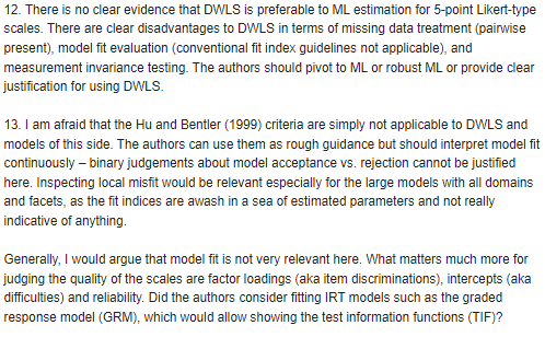
Reviewer 2

Data quality checks (before fitting)

Before you run WLSMV / ordinal CFA, check:

Category frequencies
Any category with very few responses? (e.g., < 5% or tiny counts)
Empty / near-empty pairs
Some item pairs may have empty cells in their K×K tables → unstable polychorics
Extreme skew / floor–ceiling
Items with almost everyone in the same category carry little information
Too many categories for N
Many categories + modest sample size → sparse tables and unstable estimation

If you see sparse categories, consider collapsing adjacent categories (with a substantive rationale).

What to do if categories are sparse

Options (in order of “least invasive”):

Collapse adjacent categories (e.g., merge 1–2 or 4–5)
- do it consistently across groups/time if you’ll test invariance
Drop an item that is essentially constant or unusable
Collect more data (sparse tables are fundamentally a sample-size problem)

Avoid “data-driven collapsing” that changes the construct meaning. Document the decision clearly.

MG-CFA-ordinal

Prerequisites

When we test multigroup invariance with ordinal data we assume that the THRESHOLDS are also equal between the two groups, but before running the analysis, remember:

the number of parameters is higher than with continuous data…and you split the data in two or more parts! Be sure you have enough data in each group
all the observed indicators hold the same categories in each group, otherwise you cannot fit the model

Steps

The steps that you should follow fo MG-CFA with ordinal data are slightly different:

Baseline model, as the configural model
Equal thresholds model, you should start by forcing the thresholds to be equal across groups
Equal loadings and thresholds model, only now you can fix the loadings to be equal across groups

In `R`

I use again the adaptability items. I manually added a group variable.

D.ad$group <- c(rep("G1", 428), rep("G2", 1083-428))
# 1. FIT THE BASELINE/CONFIGURAL MODEL
fConf <- sem(mOrd, D.ad, std.lv=T,
             ordered = T, group = "group")
# 2. FIT THE FIXED THRESHOLDS MODEL
fTresh<- sem(mOrd, D.ad, std.lv=T,
             ordered = T, group = "group",
             group.equal = c("thresholds"))
# 3. FIT THE FIXED LOADINGS MODEL
fLoad <- sem(mOrd, D.ad, std.lv=T,
             ordered = T, group = "group",
             group.equal = c("thresholds", "loadings"))

Model fit comparison

fi <- c("cfi", "tli", "srmr", "rmsea", "bic", "aic",
        "cfi.scaled","tli.scaled","rmsea.scaled")
fitTable <- rbind(fitmeasures(fConf, fi),
                  fitmeasures(fTresh, fi),
                  fitmeasures(fLoad, fi))

	cfi	tli	srmr	rmsea	bic	aic	cfi.scaled	tli.scaled	rmsea.scaled
baseline	0.987	0.981	0.045	0.062	NA	NA	0.957	0.940	0.083
thresholds	0.988	0.991	0.045	0.043	NA	NA	0.961	0.971	0.058
loadings	0.988	0.991	0.045	0.042	NA	NA	0.965	0.975	0.053

In multigroup ordinal SEM, robust fit indices are preferable in principle, but they are not always available in practice. When they disappear, scaled indices are the fallback (but less satisfactory)

Model results

Group 1					Group 2
lhs	op	rhs	est	\|\|	lhs	op	rhs	est
Loadings
cb	=~	Adaptability_1	0.70	\|\|	cb	=~	Adaptability_1	0.66
cb	=~	Adaptability_2	0.69	\|\|	cb	=~	Adaptability_2	0.66
cb	=~	Adaptability_3	0.69	\|\|	cb	=~	Adaptability_3	0.64
cb	=~	Adaptability_4	0.54	\|\|	cb	=~	Adaptability_4	0.56
cb	=~	Adaptability_5	0.66	\|\|	cb	=~	Adaptability_5	0.58
cb	=~	Adaptability_6	0.65	\|\|	cb	=~	Adaptability_6	0.49
em	=~	Adaptability_7	0.68	\|\|	em	=~	Adaptability_7	0.66
em	=~	Adaptability_8	0.68	\|\|	em	=~	Adaptability_8	0.69
em	=~	Adaptability_9	0.71	\|\|	em	=~	Adaptability_9	0.65
Latent covariance
cb	~~	em	0.62	\|\|	cb	~~	em	0.55
Thresholds
Adaptability_1	\|	t1	-2.13	\|\|	Adaptability_1	\|	t1	-2.11
Adaptability_1	\|	t2	-1.69	\|\|	Adaptability_1	\|	t2	-1.62
Adaptability_1	\|	t3	-1.06	\|\|	Adaptability_1	\|	t3	-1.05
Adaptability_1	\|	t4	-0.36	\|\|	Adaptability_1	\|	t4	-0.30
Adaptability_1	\|	t5	0.52	\|\|	Adaptability_1	\|	t5	0.48
Adaptability_1	\|	t6	1.14	\|\|	Adaptability_1	\|	t6	1.21

Additional materials

Svetina et al. (Svetina et al., 2020) tutorial, suggestions, and model fit recommendations for MG-CFA with ordinal data
Enrico Perinelli held a psicostat meeting on the topic following Svetina et al.’s code [slides](https://psicostat.dpss.psy.unipd.it/meetings/slides/2022-06-17_perinelli.pdf)

Exercises → Lab

Open and work through:

labs/lab08_ordinal_sem_invariance.qmd link

Focus on:

fitting the same CFA/SEM treating items as continuous vs ordered
inspecting thresholds and (polychoric) correlations
MG-CFA steps with ordinal indicators (thresholds → thresholds + loadings)

Take-home summary

Three things to remember:

Ordinal items are usually modeled via an underlying continuous latent response + thresholds
Estimation changes (DWLS/WLSMV/ULS), and fit indices are not “plug-and-play” as in ML for continuous data
With ordinal MG-CFA, threshold invariance is a key early step (often before loadings)

Acknowledgments

Thanks to Massimiliano Pastore for his slides!

References

Brauer, K., Ranger, J., & Ziegler, M. (2023). Confirmatory factor analyses in psychological test adaptation and development. Psychological Test Adaptation and Development, 4(1), 4–12. https://doi.org/10.1027/2698-1866/a000034

Li, C.-H. (2016). Confirmatory factor analysis with ordinal data: Comparing robust maximum likelihood and diagonally weighted least squares. Behavior Research Methods, 48(3), 936–949. https://doi.org/10.3758/s13428-015-0619-7

McNeish, D. (2023). Dynamic fit index cutoffs for categorical factor analysis with likert-type, ordinal, or binary responses. American Psychologist, 78(9), 1061–1075. https://doi.org/10.1037/amp0001213

Savalei, V. (2021). Improving Fit Indices in Structural Equation Modeling with Categorical Data. Multivariate Behavioral Research, 56(3), 390–407. https://doi.org/10.1080/00273171.2020.1717922

Shi, D., Maydeu-Olivares, A., & Rosseel, Y. (2020). Assessing fit in ordinal factor analysis models: SRMR vs. RMSEA. Structural Equation Modeling: A Multidisciplinary Journal, 27(1), 1–15. https://doi.org/10.1080/10705511.2019.1611434

Svetina, D., Rutkowski, L., & Rutkowski, D. (2020). Multiple-group invariance with categorical outcomes using updated guidelines: An illustration using mplus and the lavaan/semTools packages. Structural Equation Modeling: A Multidisciplinary Journal, 27(1), 111130. https://doi.org/10.1080/10705511.2019.1602776

Xia, Y., & Yang, Y. (2019). RMSEA, CFI, and TLI in structural equation modeling with ordered categorical data: The story they tell depends on the estimation methods. Behavior Research Methods, 51(1), 409–428. https://doi.org/10.3758/s13428-018-1055-2

SEM with ordinal variables

Today in the workflow

Learning objectives

Introduction

Introduction

Likert scales

The adaptability data

Wrong correlations

In lavaan and SEM

How to fit a CFA with ordinal data

Results (1)

Results (2)

Results (3)

Results (4)

Thresholds (1)

Thresholds (2)

Results (5)

Model fit

Model fit, suggestions

Reviewer 2

Data quality checks (before fitting)

What to do if categories are sparse

MG-CFA-ordinal

Prerequisites

Steps

In R

Model fit comparison

Model results

Additional materials

Exercises → Lab

Take-home summary

Acknowledgments

References

The `adaptability` data

In `lavaan` and SEM

In `R`