Longitudinal SEM: Growth + Invariance Over Time
Latent Growth Models & Measurement Invariance Across Waves
Tommaso Feraco
Today in the workflow
Specify → Identify → Estimate → Evaluate → Revise/Report
Today: measurement in a longitudinal fashion.
Growth: measuring and testing change in latent variables.
Learning objectives
By the end of today you can:
- Fit and justify measurement invariance over time (longitudinal CFA).
- Specify and estimate latent growth curve models (LGM) in SEM form.
- Interpret growth parameters (means, variances, covariances) and understand time coding.
- Use global + local diagnostics to decide on disciplined respecification.
What question are we asking?
Longitudinal SEM is not one model, but a family of models.
Tip
Choose the model family from the scientific question:
- Growth (LGM): “How do people change on average? How do trajectories differ?”
- Stability / lagged prediction (CLPM/RI-CLPM): “Do individual changes predict later changes?”
- Change processes (LCS): “How is change from t→t+1 driven/coupled?”
Today: Invariance over time + LGM (growth).
RI-CLPM and LCS are linked as extras later.
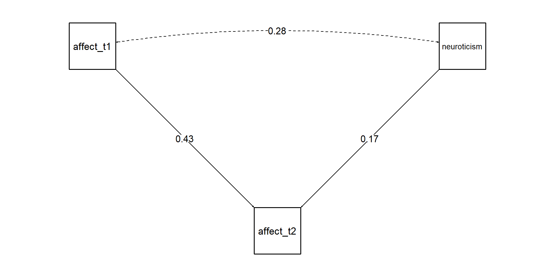
Not a longitudinal model
Warning
The intercepts problem: Without controlling for the TRUE latent variable, variables that are associated with T1 levels will always be associated with T2 level even after accounting for T1 scores. You must account for the latent intercept of that variable. T1 scores is just an indicator of that variable + some error. Which is the same for T2.
- You are not testing whether affect predicts changes in neuroticism from T1 to T2
Minimal key concept: measurement-first (two-step)
Two-step mindset
- Measurement model: is the construct measured comparably across waves?
- Structural/growth model: only then interpret change parameters.
If measurement shifts over time, “growth” can become a mixture of:
- true change in the latent construct
- changes in item functioning / scaling / intercepts
Longitudinal invariance
Longitudinal invariance steps
Measurement waves are our “groups” for the MG-CFA.
- Configural: same factor structure each wave
- Metric: equal loadings (\(Λ\)) across waves
- Scalar: equal intercepts (\(τ\)) across waves
→ necessary for latent mean / growth mean interpretation
Warning
Key point: Without at least (partial) scalar invariance, mean differences over time can be artifacts of shifting intercepts (thresholds for ordinal items).
Identification reminders (longitudinal CFA)
For each wave:
- Fix factor scale (e.g., one loading = 1, or factor variance = 1)
- With multiple waves, keep scaling consistent across time
In longitudinal CFA with means, the usual identification logic extends:
- Intercepts and factor means can’t all be free without constraints
- In lavaan, a standard way is fix factor mean at wave 1 to 0 and estimate others (or use growth factors later)
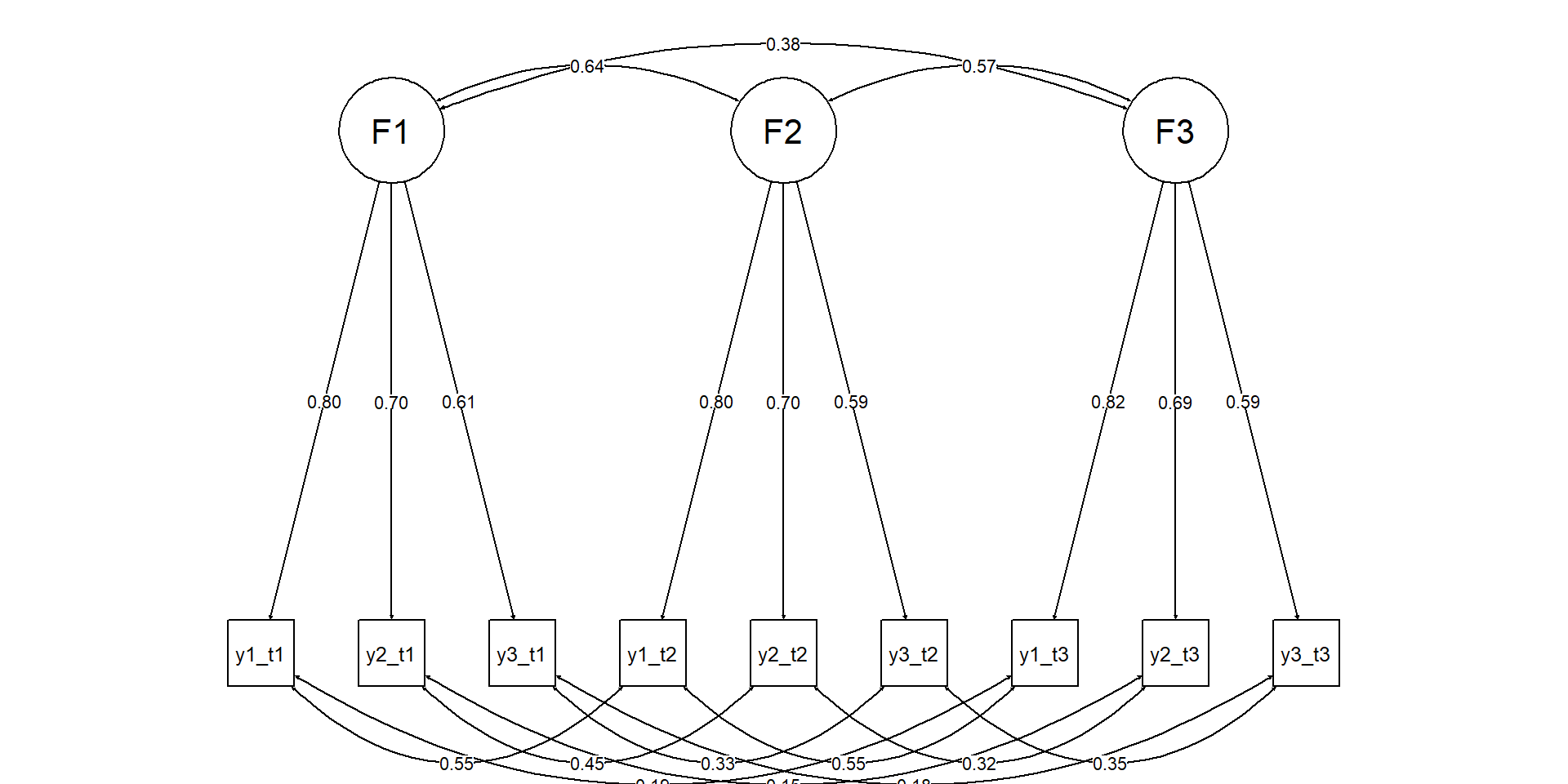
Diagram: longitudinal CFA
Live coding setup
Example data (transparent simulation)
We simulate:
- One latent trait at each wave
- Strong stability (correlated factors over time)
- Some correlated residuals for the same indicator across waves (realistic)
- Later we impose invariance constraints in fitting
Note
We set meanstructure = TRUE in simulation to generate item intercepts + means consistently with the population model.
pop <- '
# Wave 1 factor
F1 =~ 1*y1_1 + .8*y2_1 + .9*y3_1 + .7*y4_1
# Wave 2 factor
F2 =~ 1*y1_2 + .8*y2_2 + .9*y3_2 + .7*y4_2
# Wave 3 factor
F3 =~ 1*y1_3 + .8*y2_3 + .9*y3_3 + .7*y4_3
# Wave 4 factor
F4 =~ 1*y1_4 + .8*y2_4 + .9*y3_4 + .7*y4_4

# Factor means (0 baseline; increasing means)
F1 ~ 0*1
F2 ~ .2*1
F3 ~ .5*1
F4 ~ .8*1

# Factor variances
F1 ~~ 1*F1
F2 ~~ 1*F2
F3 ~~ 1*F3
F4 ~~ 1*F4

# Stability (correlations)
F1 ~~ .70*F2
F2 ~~ .75*F3
F3 ~~ .80*F4
F1 ~~ .60*F3
F2 ~~ .65*F4
F1 ~~ .55*F4

# Residual variances (items)
y1_1 ~~ .5*y1_1; y2_1 ~~ .6*y2_1; y3_1 ~~ .5*y3_1; y4_1 ~~ .7*y4_1
y1_2 ~~ .5*y1_2; y2_2 ~~ .6*y2_2; y3_2 ~~ .5*y3_2; y4_2 ~~ .7*y4_2
y1_3 ~~ .5*y1_3; y2_3 ~~ .6*y2_3; y3_3 ~~ .5*y3_3; y4_3 ~~ .7*y4_3
y1_4 ~~ .5*y1_4; y2_4 ~~ .6*y2_4; y3_4 ~~ .5*y3_4; y4_4 ~~ .7*y4_4

# Correlated residuals across adjacent waves for same indicator
# (method/wording carryover)
y1_1 ~~ .25*y1_2
y1_2 ~~ .25*y1_3
y1_3 ~~ .25*y1_4
y2_1 ~~ .20*y2_2
y2_2 ~~ .20*y2_3
y2_3 ~~ .20*y2_4
'

dat <- simulateData(pop, sample.nobs = 6000, meanstructure = TRUE)
Step 1: Configural longitudinal CFA
We specify one factor per wave, same indicators each wave.
We also allow conceptually justified correlated residuals (same items).
mod_config <- '
F1 =~ y1_1 + y2_1 + y3_1 + y4_1
F2 =~ y1_2 + y2_2 + y3_2 + y4_2
F3 =~ y1_3 + y2_3 + y3_3 + y4_3
F4 =~ y1_4 + y2_4 + y3_4 + y4_4

# correlated residuals for the same item across adjacent waves
y1_1 ~~ y1_2
y1_2 ~~ y1_3
y1_3 ~~ y1_4
y2_1 ~~ y2_2
y2_2 ~~ y2_3
y2_3 ~~ y2_4
'

fit_config <- cfa(mod_config, data = dat, meanstructure = TRUE)
fitMeasures(fit_config, c("chisq","df","cfi","tli","rmsea","srmr"))
chisq df cfi tli rmsea srmr
85.683 92.000 1.000 1.000 0.000 0.007 Step 2: Metric invariance: equal loadings
mod_metric <- '
# equal loadings across timepoints
F1 =~ l1*y1_1 + l2*y2_1 + l3*y3_1 + l4*y4_1
F2 =~ l1*y1_2 + l2*y2_2 + l3*y3_2 + l4*y4_2
F3 =~ l1*y1_3 + l2*y2_3 + l3*y3_3 + l4*y4_3
F4 =~ l1*y1_4 + l2*y2_4 + l3*y3_4 + l4*y4_4

# correlated residuals
y1_1 ~~ y1_2
y1_2 ~~ y1_3
y1_3 ~~ y1_4
y2_1 ~~ y2_2
y2_2 ~~ y2_3
y2_3 ~~ y2_4
'

fit_metric <- cfa(mod_metric, data = dat, meanstructure = TRUE)
Note
We are not using the group= argument because data are wide.
Step 3: Scalar invariance: equal intercepts too
mod_scalar <- '
# equal loadings across timepoints
F1 =~ l1*y1_1 + l2*y2_1 + l3*y3_1 + l4*y4_1
F2 =~ l1*y1_2 + l2*y2_2 + l3*y3_2 + l4*y4_2
F3 =~ l1*y1_3 + l2*y2_3 + l3*y3_3 + l4*y4_3
F4 =~ l1*y1_4 + l2*y2_4 + l3*y3_4 + l4*y4_4

# equal intercepts across time
y1_1 ~ i1*1; y1_2 ~ i1*1; y1_3 ~ i1*1; y1_4 ~ i1*1
y2_1 ~ i2*1; y2_2 ~ i2*1; y2_3 ~ i2*1; y2_4 ~ i2*1
y3_1 ~ i3*1; y3_2 ~ i3*1; y3_3 ~ i3*1; y3_4 ~ i3*1
y4_1 ~ i4*1; y4_2 ~ i4*1; y4_3 ~ i4*1; y4_4 ~ i4*1

# correlated residuals
y1_1 ~~ y1_2
y1_2 ~~ y1_3
y1_3 ~~ y1_4
y2_1 ~~ y2_2
y2_2 ~~ y2_3
y2_3 ~~ y2_4

# free means
F1 ~ 0*1
F2 ~ m2*1
F3 ~ m3*1
F4 ~ m4*1
'
fit_scalar <- cfa(mod_scalar, data = dat, meanstructure = TRUE)
Tip
Freeing means could be essential if there is actual mean change.
Evaluate invariance: fit comparisons
Chi-Squared Difference Test

            Df    AIC    BIC Chisq Chisq diff   RMSEA Df diff Pr(>Chisq)
fit_config  92 246326 246728  85.7
fit_metric 101 246315 246657  92.7       7.06 0.00000       9       0.63
fit_scalar 110 246309 246591 105.3 12.57 0.00813 9 0.18data.frame(bind_rows(
config = fitMeasures(fit_config, c("cfi","rmsea","srmr")),
metric = fitMeasures(fit_metric, c("cfi","rmsea","srmr")),
scalar = fitMeasures(fit_scalar, c("cfi","rmsea","srmr")),.id = "model")) model cfi rmsea srmr
1 config 1 0 0.00684
2 metric 1 0 0.00891
3 scalar 1 0 0.00929Tip
Always check where misfit arises (local diagnostics).
Diagnostics: global vs local fit (in invariance)
Global: χ², CFI/TLI, RMSEA (+CI), SRMR
Local:
- standardized residuals
- modification indices (MI)
- inspect which items/waves break invariance
# Local diagnostics example
mi <- modificationIndices(fit_scalar)
mi |> arrange(desc(mi)) |> head(10)
lhs op rhs mi epc sepc.lv sepc.all sepc.nox
1 y1_1 ~~ y4_1 7.95 -0.027 -0.027 -0.044 -0.044
2 F2 =~ y1_1 5.27 0.027 0.027 0.022 0.022
3 F3 =~ y1_1 5.03 0.024 0.023 0.019 0.019
4 F2 =~ y4_1 3.95 -0.025 -0.025 -0.023 -0.023
5 F1 =~ y4_4 3.75 0.025 0.025 0.023 0.023
6 y4_3 ~~ y2_4 3.70 0.017 0.017 0.026 0.026
7 F1 =~ y4_3 3.56 -0.024 -0.024 -0.023 -0.023
8 F2 =~ y4_4 3.45 0.024 0.024 0.022 0.022
9 y3_1 ~~ y4_3 3.31 -0.017 -0.017 -0.028 -0.028
10 y4_1 ~~ y2_2 3.17 -0.015 -0.015 -0.023 -0.023Pitfall/callout: “Partial invariance = fishing?”
Warning
Partial invariance is not “cheating” if done transparently:
- free the smallest number of parameters
- justify based on item content / design changes
- report which parameters were freed
- verify conclusions are robust (sensitivity)
A good practice: free one intercept (or loading) at a time guided by theory + MI, then reassess.
From time invariance to growth
Transition: from invariance to growth
If longitudinal (partial) scalar invariance holds, we can interpret latent means over time (like we did for group comparisons in MG-CFA).
Growth models re-express these latent means as a trajectory using growth factors:
- Intercept factor (i): baseline level (at a chosen time point)
- Slope factor (s): rate of change (linear, unless extended)
- Optional: quadratic slope, piecewise slopes…
Transition: from invariance to growth
What questions do you answer with latent growth models?
- What is the average trajectory for all respondents?
- What is their initial value (i.e., mean)?
- Is there any change?
- What’s the form of the change
- Is the average trajectory enough or participants vary in their trajectories?
- random effects of intercepts and slope
- Are random effects explainable? How? Do we need more variables?
Minimal math: LGM as CFA with time scores
For person n at time t:
\[ \eta_{nt} = i_n + \lambda_t s_n + \varepsilon_{nt} \]
- \((i_n)\) and \((s_n)\) are latent variables (random effects)
- \((\lambda_t)\) are fixed time scores (e.g., 0,1,2,3)
- \((\varepsilon_{nt})\) are time-specific residuals
Means and variances:
- \((E(i_n) = \mu_i)\), \((Var(i_n)=\sigma_i^2)\)
- \((E(s_n) = \mu_s)\), \((Var(s_n)=\sigma_s^2)\)
- \((Cov(i_n,s_n)=\sigma_{is})\)
Diagram: growth model (intercept + slope)
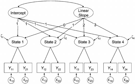
Note
This is a linear second-order latent growth curve model
LGM on observed composites
We’ll start with a simple observed repeated measure (think: scale score).
In practice, you often combine:
- longitudinal invariance CFA for measurement
- then growth model on latent factors (“second-order” growth)
Create an observed score per wave from the data we used before:
Warning
(teaching-friendly less publication/SEM-friendly)
Linear growth model in lavaan
In lavaan, growth() is a convenience wrapper that fits an SEM with meanstructure=TRUE by default (needed to estimate growth means). If you use sem()/cfa(), you must set it explicitly.
Warning
This model is already assuming random intercepts and slopes
The growth summary
lavaan 0.6-19 ended normally after 26 iterations

  Estimator                                         ML
  Optimization method                           NLMINB
  Number of model parameters                        12

  Number of observations                          6000

Model Test User Model:

  Test statistic                                39.720
  Degrees of freedom                                 2
  P-value (Chi-square)                           0.000

Model Test Baseline Model:

  Test statistic                             10572.830
  Degrees of freedom                                 6
  P-value                                        0.000

User Model versus Baseline Model:

  Comparative Fit Index (CFI)                    0.996
  Tucker-Lewis Index (TLI)                       0.989

Loglikelihood and Information Criteria:

  Loglikelihood user model (H0)             -26907.698
  Loglikelihood unrestricted model (H1)     -26887.838

  Akaike (AIC)                               53839.396
  Bayesian (BIC)                             53919.790
  Sample-size adjusted Bayesian (SABIC)      53881.658

Root Mean Square Error of Approximation:

  RMSEA                                          0.056
  90 Percent confidence interval - lower         0.042
  90 Percent confidence interval - upper         0.072
  P-value H_0: RMSEA <= 0.050                    0.230
  P-value H_0: RMSEA >= 0.080                    0.006

Standardized Root Mean Square Residual:

  SRMR                                           0.014

Parameter Estimates:

  Standard errors                             Standard
  Information                                 Expected
  Information saturated (h1) model          Structured

Latent Variables:
                   Estimate  Std.Err  z-value  P(>|z|)   Std.lv  Std.all
  i =~
    y_t1              1.000                               0.691    0.742
    y_t2              1.000                               0.691    0.741
    y_t3              1.000                               0.691    0.750
    y_t4              1.000                               0.691    0.756
  s =~
    y_t1              0.000                               0.000    0.000
    y_t2              1.000                               0.175    0.187
    y_t3              2.000                               0.350    0.379
    y_t4              3.000                               0.524    0.574

Covariances:
                   Estimate  Std.Err  z-value  P(>|z|)   Std.lv  Std.all
 .y_t1 ~~
   .y_t2              0.084    0.014    5.812    0.000    0.084    0.208
 .y_t2 ~~
   .y_t3              0.102    0.007   15.354    0.000    0.102    0.262
 .y_t3 ~~
   .y_t4              0.065    0.015    4.253    0.000    0.065    0.218
  i ~~
    s                -0.028    0.009   -3.213    0.001   -0.228   -0.228

Intercepts:
                   Estimate  Std.Err  z-value  P(>|z|)   Std.lv  Std.all
    i                -0.017    0.012   -1.473    0.141   -0.025   -0.025
    s                 0.230    0.004   56.514    0.000    1.317    1.317

Variances:
                   Estimate  Std.Err  z-value  P(>|z|)   Std.lv  Std.all
   .y_t1              0.390    0.024   16.180    0.000    0.390    0.449
   .y_t2              0.418    0.014   29.997    0.000    0.418    0.480
   .y_t3              0.359    0.014   26.593    0.000    0.359    0.423
   .y_t4              0.248    0.025    9.774    0.000    0.248    0.297
    i                 0.478    0.025   19.414    0.000    1.000    1.000
    s                 0.031    0.005    6.415    0.000    1.000    1.000
Interpreting the growth output
Key parameters:
- Mean(i) = average baseline (at time score 0)
- Mean(s) = average change per time unit
- Var(i) = between-person differences in baseline
- Var(s) = between-person differences in change (heterogeneity)
- Cov(i,s) = association between intercept and slope (often negative due to artifacts: regression-to-mean, boundaries, heteroskedasticity - interpret carefully)
  lhs op rhs    est    se     z pvalue ci.lower ci.upper
1   i ~~   i  0.478 0.025 19.41  0.000    0.429    0.526
2   s ~~   s  0.031 0.005  6.42  0.000    0.021    0.040
3   i ~~   s -0.028 0.009 -3.21  0.001   -0.044   -0.011
4   i ~1     -0.017 0.012 -1.47  0.141   -0.040    0.006
5   s ~1      0.230 0.004 56.51  0.000    0.222    0.238
Pitfall/callout: time coding is a modeling choice
Warning
Changing time scores changes interpretation.
If you code slope loadings as 0,1,2,3 then:
- intercept = expected value at wave 1
If you code as -1,0,1,2 then: - intercept = expected value at wave 2
If you center at the midpoint, intercept becomes “midpoint status.”
Remember to choose a centering that matches the substantive interpretation you want.
Warning
TIME POINTS MUST BE CHOSEN A PRIORI, BASED ON THEORY.
e.g. Is this time point large enough to see change?
A stepwise approach to LGM
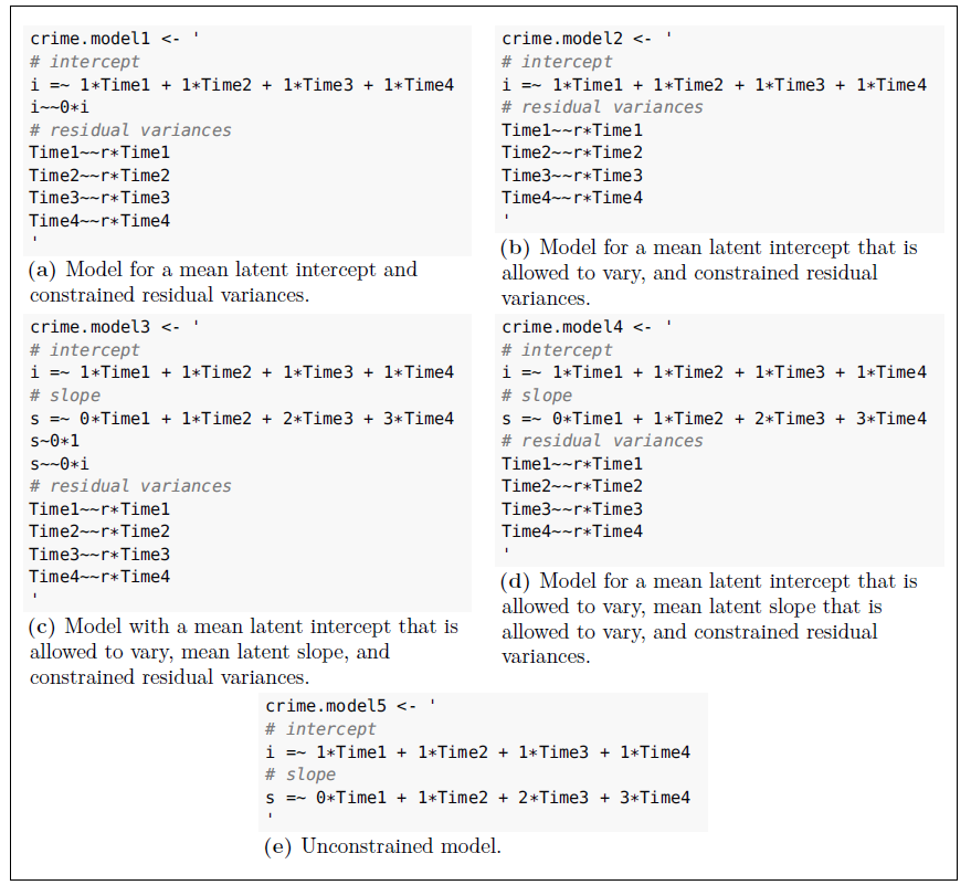

Beaujean (2014)
LGM extensions
The second-order factor model
The measurement block
lgm_linear_2ndorder <- '
## 1) MEASUREMENT (strong/scalar invariance)

# equal loadings across time (metric invariance)
F1 =~ 1*y1_1 + l2*y2_1 + l3*y3_1 + l4*y4_1
F2 =~ 1*y1_2 + l2*y2_2 + l3*y3_2 + l4*y4_2
F3 =~ 1*y1_3 + l2*y2_3 + l3*y3_3 + l4*y4_3
F4 =~ 1*y1_4 + l2*y2_4 + l3*y3_4 + l4*y4_4

# equal intercepts across time (scalar invariance)
y1_1 ~ i1*1; y1_2 ~ i1*1; y1_3 ~ i1*1; y1_4 ~ i1*1
y2_1 ~ i2*1; y2_2 ~ i2*1; y2_3 ~ i2*1; y2_4 ~ i2*1
y3_1 ~ i3*1; y3_2 ~ i3*1; y3_3 ~ i3*1; y3_4 ~ i3*1
y4_1 ~ i4*1; y4_2 ~ i4*1; y4_3 ~ i4*1; y4_4 ~ i4*1

# (optional) correlated residuals across waves
y1_1 ~~ r1*y1_2
y1_2 ~~ r1*y1_3
y1_3 ~~ r1*y1_4

y2_1 ~~ r2*y2_2
y2_2 ~~ r2*y2_3
y2_3 ~~ r2*y2_4

y3_1 ~~ r3*y3_2
y3_2 ~~ r3*y3_3
y3_3 ~~ r3*y3_4

y4_1 ~~ r4*y4_2
y4_2 ~~ r4*y4_3
y4_3 ~~ r4*y4_4

'
The latent change block
lgm_linear_2ndorder <- '
## 2) SECOND-ORDER GROWTH ON LATENT FACTORS

# growth factors (second-order)
i =~ 1*F1 + 1*F2 + 1*F3 + 1*F4
s =~ 0*F1 + 1*F2 + 2*F3 + 3*F4

# estimate growth means (trajectory in the latent metric)
i ~ 1
s ~ 1

# fix means of the first-order factors so i/s carry the mean structure
F1 ~ 0*1
F2 ~ 0*1
F3 ~ 0*1
F4 ~ 0*1

# (optional) allow i-s covariance
i ~~ s

# (optional) residual autocorrelation among the time-specific factors
F1 ~~ F2
F2 ~~ F3
F3 ~~ F4
'
fit_lgm_2nd <- sem(lgm_linear_2ndorder, data = dat, meanstructure = TRUE)
Warning
We are not using growth() here but sem + meanstructure=TRUE
Quadratic growth example (simulation)
set.seed(123)

## ----------------------------
## 1) Population model: quadratic growth on observed variables
## ----------------------------
pop_quad <- '
# Growth factors (no first-order measurement factors; y_t* are the repeated measures)
i =~ 1*y_t1 + 1*y_t2 + 1*y_t3 + 1*y_t4
s =~ 0*y_t1 + 1*y_t2 + 2*y_t3 + 3*y_t4
q =~ 0*y_t1 + 1*y_t2 + 4*y_t3 + 9*y_t4

# Factor means (imply the mean trajectory)
i ~ 0*1
s ~ 0.40*1
q ~ 0.15*1

# Factor (co)variances (individual differences)
i ~~ 1.00*i
s ~~ 0.40*s
q ~~ 0.10*q
i ~~ 0.30*s
i ~~ 0.10*q
s ~~ 0.05*q

# Fix observed intercepts so means come from i,s,q
y_t1 ~ 0*1
y_t2 ~ 0*1
y_t3 ~ 0*1
y_t4 ~ 0*1

# Residual variances
y_t1 ~~ 0.64*y_t1
y_t2 ~~ 0.64*y_t2
y_t3 ~~ 0.64*y_t3
y_t4 ~~ 0.64*y_t4

# Adjacent residual autocorrelation (covariances)
y_t1 ~~ 0.192*y_t2
y_t2 ~~ 0.192*y_t3
y_t3 ~~ 0.192*y_t4
'

dat <- simulateData(pop_quad, sample.nobs = 6000, meanstructure = TRUE)
Quadratic results
## ----------------------------
## 2) FIT LGM without quadratic
## ----------------------------
lgm_lin <- '
i =~ 1*y_t1 + 1*y_t2 + 1*y_t3 + 1*y_t4
s =~ 0*y_t1 + 1*y_t2 + 2*y_t3 + 3*y_t4
'

fit_lin <- growth(lgm_lin, data = dat)

fitMeasures(fit_lin,  c("cfi","tli","rmsea","srmr","aic","bic"))
cfi tli rmsea srmr aic bic
0.929 0.915 0.242 0.106 84653.539 84713.835 ## ----------------------------
## 3) FIT LGM with quadratic
## ----------------------------
lgm_quad <- '
i =~ 1*y_t1 + 1*y_t2 + 1*y_t3 + 1*y_t4
s =~ 0*y_t1 + 1*y_t2 + 2*y_t3 + 3*y_t4
q =~ 0*y_t1 + 1*y_t2 + 4*y_t3 + 9*y_t4
'
fit_quad <- growth(lgm_quad, data = dat)
fitMeasures(fit_quad, c("cfi","tli","rmsea","srmr","aic","bic")) cfi tli rmsea srmr aic bic
1.000 1.000 0.008 0.001 82904.604 82991.697
Chi-Squared Difference Test

         Df   AIC   BIC   Chisq Chisq diff RMSEA Df diff          Pr(>Chisq)
fit_quad  1 82905 82992    1.42
fit_lin   5 84654 84714 1758.36       1757  0.27       4 <0.0000000000000002

fit_quad
fit_lin  ***
---
Signif. codes:  0 '***' 0.001 '**' 0.01 '*' 0.05 '.' 0.1 ' ' 1
Conditional growth: predictors of i and s
Add a time-invariant covariate x predicting baseline and growth.
Summary of the conditional model
lavaan 0.6-19 ended normally after 41 iterations

  Estimator                                         ML
  Optimization method                           NLMINB
  Number of model parameters                        14

  Number of observations                          6000

Model Test User Model:

  Test statistic                               502.347
  Degrees of freedom                                 4
  P-value (Chi-square)                           0.000

Model Test Baseline Model:

  Test statistic                             24670.853
  Degrees of freedom                                10
  P-value                                        0.000

User Model versus Baseline Model:

  Comparative Fit Index (CFI)                    0.980
  Tucker-Lewis Index (TLI)                       0.949

Loglikelihood and Information Criteria:

  Loglikelihood user model (H0)             -41685.211
  Loglikelihood unrestricted model (H1)     -41434.038

  Akaike (AIC)                               83398.422
  Bayesian (BIC)                             83492.216
  Sample-size adjusted Bayesian (SABIC)      83447.727

Root Mean Square Error of Approximation:

  RMSEA                                          0.144
  90 Percent confidence interval - lower         0.134
  90 Percent confidence interval - upper         0.155
  P-value H_0: RMSEA <= 0.050                    0.000
  P-value H_0: RMSEA >= 0.080                    1.000

Standardized Root Mean Square Residual:

  SRMR                                           0.052

Parameter Estimates:

  Standard errors                             Standard
  Information                                 Expected
  Information saturated (h1) model          Structured

Latent Variables:
                   Estimate  Std.Err  z-value  P(>|z|)   Std.lv  Std.all
  i =~
    y_t1              1.000                               0.542    0.420
    y_t2              1.000                               0.542    0.315
    y_t3              1.000                               0.542    0.197
    y_t4              1.000                               0.542    0.121
  s =~
    y_t1              0.000                               0.000    0.000
    y_t2              1.000                               0.832    0.483
    y_t3              2.000                               1.664    0.605
    y_t4              3.000                               2.496    0.557

Regressions:
                   Estimate  Std.Err  z-value  P(>|z|)   Std.lv  Std.all
  i ~
    x                -0.012    0.016   -0.775    0.438   -0.022   -0.022
  s ~
    x                 0.030    0.014    2.138    0.033    0.036    0.036

Covariances:
                   Estimate  Std.Err  z-value  P(>|z|)   Std.lv  Std.all
 .y_t1 ~~
   .y_t2              0.416    0.028   14.784    0.000    0.416    0.688
 .y_t2 ~~
   .y_t3             -0.248    0.020  -12.374    0.000   -0.248   -0.465
 .y_t3 ~~
   .y_t4              2.814    0.104   27.025    0.000    2.814    0.935
 .i ~~
   .s                 0.857    0.037   22.944    0.000    1.900    1.900

Intercepts:
                   Estimate  Std.Err  z-value  P(>|z|)   Std.lv  Std.all
   .i                -0.141    0.016   -9.050    0.000   -0.259   -0.259
   .s                 0.630    0.014   44.449    0.000    0.757    0.757

Variances:
                   Estimate  Std.Err  z-value  P(>|z|)   Std.lv  Std.all
   .y_t1              1.373    0.058   23.604    0.000    1.373    0.823
   .y_t2              0.266    0.027    9.840    0.000    0.266    0.090
   .y_t3              1.073    0.065   16.476    0.000    1.073    0.142
   .y_t4              8.445    0.223   37.805    0.000    8.445    0.420
   .i                 0.294    0.053    5.575    0.000    1.000    1.000
   .s                 0.692    0.028   24.380    0.000    0.999    0.999
Warning
As for \(i\) ~~ \(s\) correlations, when an external variable is associated with the intercept, it will probably be associated with the slope, but this is often an artifact. A second-order model could help resolving this issue and avoid issues due to bounds in measures.
Local diagnostics for growth models
Global fit is necessary but not sufficient.
- residual autocorrelation (y_t2 ~~ y_t3, etc.)
- MIs suggesting additional residual correlations
- implausible negative variances (Heywood)
- standardized residuals / fitted vs observed means
    lhs op  rhs   mi    epc sepc.lv sepc.all sepc.nox
1     i =~ y_t4 1.42  4.525   5.596    1.267    1.267
2     i =~ y_t3 1.42 -1.508  -1.865   -0.682   -0.682
3     i =~ y_t2 1.42  1.508   1.865    1.084    1.084
4     s =~ y_t1 1.42  0.099   0.108    0.084    0.084
5  y_t2 ~1      1.42 -0.014  -0.014   -0.008   -0.008
6     s =~ y_t2 1.42 -0.033  -0.036   -0.021   -0.021
7  y_t1 ~1      1.42  0.041   0.041    0.032    0.032
8     q =~ y_t4 1.42 -0.281  -0.121   -0.027   -0.027
9     q =~ y_t1 1.42  0.281   0.121    0.094    0.094
10 y_t3 ~1      1.42  0.014   0.014    0.005    0.005
What we did NOT do (on purpose)
RI-CLPM and LCS families (they answer different questions)
Not yet available extras
→ RI-CLPM warnings & alternatives:
extras/riclpm_vs_clpm.qmd→ Latent change score models:
extras/latent-change-score_models.qmd
Exercises → Lab09
In Lab09 (link) you will:
- Longitudinal invariance ladder
- Fit configural → metric → scalar
- Decide if partial scalar is needed (and document what you free)
- Fit linear LGM (time scores 0,1,2,3)
- Interpret mean/variance of intercept and slope
- Re-center time to change intercept meaning
- Add curvature or residual autocorrelation
- Compare fit + interpretability (don’t respecify blindly)
- Conditional growth
- Add a predictor of intercept and slope; interpret effects
Take-home summary: 3 things
- Measurement invariance over time is the entry ticket to interpreting mean change.
- Growth models are SEMs with time-coded loadings: interpretation depends on time coding/centering.
- Diagnostics matter: combine global fit with local checks; respecify with theory and transparency.
References
Beaujean, A. A. (2014). Latent variable modeling using r: A step-by-step guide. Routledge. https://doi.org/10.4324/9781315869780