Multilevel Confirmatory Factor Analysis
Introduction, syntax, and practical examples in lavaan
Acknowledgments
Thanks to Luca Menghini for his slides!

Tip
If you really need anything about multilevel SEM ask Luca!
Today in the workflow
Specify → Identify → Estimate → Evaluate → Revise / Report
Focus today: what changes when data are clustered (schools/teams) or repeated (ESM / within-person).
Key idea: with clustering we need to model two covariance structures (within & between).
Learning objectives
By the end you should be able to:
- Diagnose non-independence (clusters / repeated measures) and why it matters
- Explain within vs between covariance (and how to compute them)
- Fit a two-level CFA in
lavaan(level:blocks +cluster=) - Read level-specific fit (especially
srmr_withinvssrmr_between) - Understand cross-level invariance and its link to construct meaning (e.g., traits as distributions of states)
Multilevel CFA
Multilevel what!?
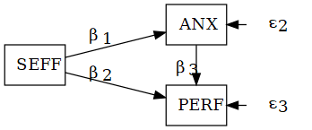
SEM = multivariate linear models formalized as systems of equations.
linear models
\(\text{PERF}=\beta_1\text{IQ}+\beta_2\text{ANX}+\epsilon\)
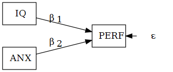
SEM system
\[ \begin{aligned} \text{ANX} &= \beta_1\text{SEFF} + \epsilon_2\\ \text{PERF} &= \beta_2\text{SEFF} + \beta_3\text{ANX} + \epsilon_3 \end{aligned} \]
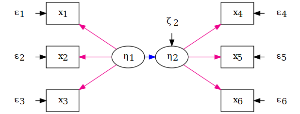
The two fundamental parts of a SEM
- Structural model: relations among variables (latent/observed)
- Measurement model: indicators → latent variables (CFA)
Confirmatory factor analysis (CFA)
CFA is the measurement model:
- number of factors (1, 2, …, k)
- which indicators load on which factor
- (co)variances among factors and residual variances

Factor structure (concept)
A factor structure is one possible configuration of relations between a set of observed variables and one or more latent factors, defining:
- the number of latent variables (1-factor, 2-factor, …, k-factor model)
- the pattern of relations between each observed variable and its factor (loading pattern)

Starting from the covariance matrix of observed variables, CFA tests the fit of one or more hypothesized factor structures and estimates the corresponding loadings.
The starting point: variance–covariance matrix
SEM is about reproducing the observed covariance matrix.
\[ H_0:\ \hat{\Sigma}(\theta) = \Sigma \]
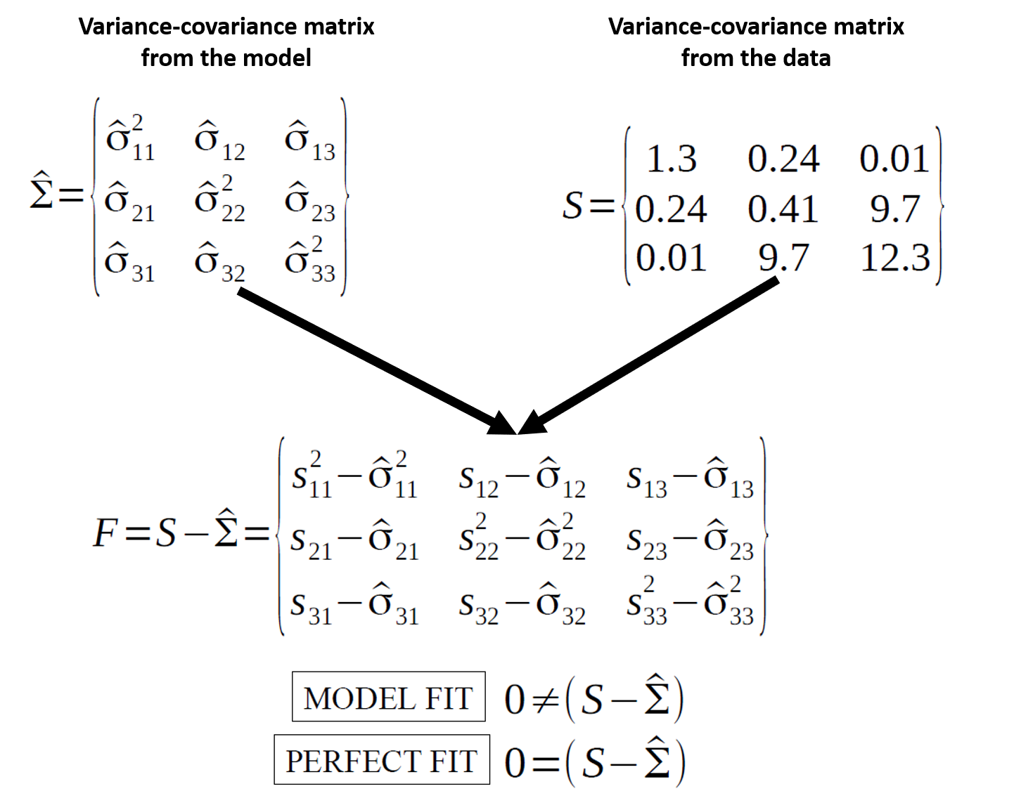
Fit indices summarize “how close” the model-implied covariance structure is to the data.
What if data are multilevel?
When observations are nested (e.g., students in classes; employees in teams) or repeated (ESM):
- local dependence: units in the same cluster/person are more similar
- independence assumption fails
- ignoring clustering can bias standard errors and sometimes distort inference
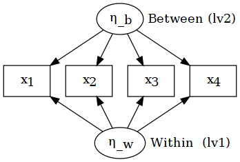
Decomposing (co)variance: within vs between
We decompose the covariance structure into:
- Between (L2): covariance among cluster means
wide <- aggregate(
  cbind(x1, x2) ~ cluster,
  data = df, FUN = mean)
names(wide)[2:3] <- c("x1.b","x2.b")

head(wide)
cluster x1.b x2.b
1 1 0.44715272 -0.20081574
2 2 -0.05879404 0.56914554
3 3 0.04562658 -0.18284200
4 4 -0.46868830 0.01981214do clusters with higher mean \((X)\) also have higher mean \((Y)\)?
- Within (L1): covariance among deviations from cluster means
df2 <- merge(df, wide, by = "cluster")
df2$x1.w <- df2$x1 - df2$x1.b
df2$x2.w <- df2$x2 - df2$x2.b

round(head(df2),2)
cluster x1 x2 x1.b x2.b x1.w x2.w
1 1 -0.56 -0.63 0.45 -0.2 -1.01 -0.42
2 1 -0.23 -1.69 0.45 -0.2 -0.68 -1.49
3 1 1.56 0.84 0.45 -0.2 1.11 1.04
4 1 0.07 0.15 0.45 -0.2 -0.38 0.35
5 1 0.13 -1.14 0.45 -0.2 -0.32 -0.94
6 1 1.72 1.25 0.45 -0.2 1.27 1.45Within: when a unit is above its cluster mean on \((X)\), is it also above its cluster mean on \((Y)\)?
Level-specific covariance matrices
- Between (L2): covariance among cluster means
            x1.b        x2.b
x1.b  0.14161724 -0.04636824
x2.b -0.04636824  0.12918010
do clusters with higher mean \((X)\) also have higher mean \((Y)\)?
Multilevel CFA (MCFA)
MCFA estimates measurement structure at both levels and matches both matrices:
within-level factor model
- \((S_\text{within}\) vs \(\hat{\Sigma}_\text{within})\)
between-level factor model
- \((S_\text{between}\) vs \(\hat{\Sigma}_\text{between})\)
That is why we need level-specific fit and level-specific parameters.
And we can ask:
- are loadings stronger at L2?
- is fit acceptable within and between?
- is the construct “the same” across levels? (cross-level invariance)
Multilevel CFA - coding
MCFA in lavaan: syntax
Two key ingredients:
level: 1andlevel: 2blocks
cluster = "cluster_id"incfa()/sem()
Simulate an ESM-like dataset
- 139 individuals
- 21 measurements each (3 days × 7 prompts/day)
- 4 Likert indicators of “Task Demand”
n_id <- 139
n_rep <- 21
N <- n_id * n_rep
ID <- rep(sprintf("S%03d", 1:n_id),
          each = n_rep)
# Between-person factor
eta_b <- rnorm(n_id, 0, 0.7)
eta_b_long <- rep(eta_b, each = n_rep)
# Within-person factor
eta_w <- rnorm(N, 0, 1.0)

lambda <- c(0.80, 0.70, 0.75, 0.65)
eps_sd <- c(0.70, 0.80, 0.75, 0.85)

y_cont <- sapply(
  seq_along(lambda),
  function(j) {
    lambda[j]*(eta_b_long + eta_w) +
      rnorm(N, 0, eps_sd[j])
})
ESMdata <- data.frame(
ID = ID,
day = rep(rep(1:3, length.out = n_rep),
times = n_id),
d1 = cut_likert(y_cont[,1]),
d2 = cut_likert(y_cont[,2]),
d3 = cut_likert(y_cont[,3]),
d4 = cut_likert(y_cont[,4])
)
head(ESMdata, 12) ID day d1 d2 d3 d4
1 S001 1 4 5 2 1
2 S001 2 4 4 5 4
3 S001 3 3 2 4 2
4 S001 1 4 4 5 5
5 S001 2 4 3 4 4
6 S001 3 2 4 4 3
7 S001 1 2 2 3 4
8 S001 2 2 4 1 5
9 S001 3 5 5 3 5
10 S001 1 4 5 4 5
11 S001 2 1 2 2 1
12 S001 3 2 3 2 2Multilevel CFA: fit the model
Multilevel CFA: level-specific fit indices
Global fit is often dominated by the within-level.
SRMR is available by level:
srmr_withinsrmr_between(key for L2 misspecification)
Multilevel CFA: level-specific parameters
   lhs op rhs est.std
1 TD_w =~  d1   0.731
2 TD_w =~  d2   0.632
3 TD_w =~  d3   0.662
4 TD_w =~ d4 0.554 lhs op rhs est.std
15 TD_b =~ d1 1.012
16 TD_b =~ d2 0.986
17 TD_b =~ d3 1.016
18 TD_b =~ d4 1.010Note: Loadings are typically stronger at the between level because measurement error tends to accumulate at Level 1 (Hox et al., 2017).
Multilevel CFA: but items are ordinal
Groups: individuals nested within groups
Subjects nested within groups
When participants belong to many groups (schools/classes/teams):
- observations are not independent
- you can still fit a single-level model, but SEs/inference can be wrong
- multilevel CFA allows separate within and between measurement models
Example: individual vs team participation
n_school <- 68
n_i <- 608
schoolID <- sample(seq_len(n_school), size = n_i, replace = TRUE)
# Between-school factor
eta_school <- rnorm(n_school, 0, 0.6)
eta_b <- eta_school[schoolID]
# Within-person factor
eta_w <- rnorm(n_i, 0, 1.0)

lam_p <- c(0.80, 0.75, 0.70, 0.65)
eps_p <- c(0.80, 0.85, 0.90, 0.95)
p_cont <- sapply(seq_along(lam_p), function(j) {
  lam_p[j] * (eta_b + eta_w) + rnorm(n_i, 0, eps_p[j])
})
edudata <- data.frame(
  schoolID = schoolID,
  p2 = cut_likert(p_cont[,1]),
  p3 = cut_likert(p_cont[,2]),
  p4 = cut_likert(p_cont[,3]),
  p5 = cut_likert(p_cont[,4])
); head(edudata, 4)
schoolID p2 p3 p4 p5
1 28 5 5 5 5
2 8 5 3 4 5
3 18 1 2 1 2
4 26 2 1 4 2Single-level CFA
Multilevel CFA: preliminary models (Level 1)
Hox (2017) suggests a preliminary check:
- fit CFA on the pooled-within covariance matrix (within-cluster centered scores)
lwd <- na.omit(edudata[, c("schoolID", paste0("p",2:5))])

ms <- data.frame(
  p2 = ave(lwd$p2, lwd$schoolID),
  p3 = ave(lwd$p3, lwd$schoolID),
  p4 = ave(lwd$p4, lwd$schoolID),
  p5 = ave(lwd$p5, lwd$schoolID)
)
cs <- lwd[, 2:ncol(lwd)] - ms

pw.cov <- (cov(cs) * (nrow(lwd) - 1)) / (nrow(lwd) - nlevels(lwd$schoolID))

fit_pw <- cfa(m_ep, sample.cov = pw.cov, sample.nobs = nrow(lwd))
round(lavInspect(fit_pw, "fit")[c("chisq","df","rmsea","cfi","tli","srmr")], 3)
chisq df rmsea cfi tli srmr
5.856 2.000 0.056 0.991 0.973 0.019 Multilevel CFA: preliminary models (Level 2)
At Level 2 (between), fit benchmark models:
- Null: No structure at Level 2. If it fits well, there is no clear structure at Level 2 (classic CFA is better: no between variability)
- Independence: Fit a model with variances only. If it fits well, there is probably a structure at Level 2, but not an interesting structural model (the pooled within matrix is better)
- Saturated: Fit a saturated model with variances and covariances. If it fits well, then the construct ‘exist’ only at Level 1, while covariances at Level 2 are spurious.
Multilevel CFA: preliminary models (Level 2)
m_sat <- '
  level: 1
    p.w =~ p2 + p3 + p4 + p5
  level: 2
    p2 ~~ p2 + p3 + p4 + p5
    p3 ~~ p3 + p4 + p5
    p4 ~~ p4 + p5
    p5 ~~ p5
' # variances and covariances

fit_null <- cfa(m_null, edudata,
                cluster = "schoolID",
                estimator = "MLR")
fit_ind  <- cfa(m_ind,  edudata,
                cluster = "schoolID",
                estimator = "MLR")
fit_sat  <- cfa(m_sat,  edudata,
                cluster = "schoolID",
                estimator = "MLR")
df rmsea.robust cfi.robust srmr_within srmr_between
null 12 0.085 0.908 0.057 NA
ind 8 0.105 0.907 0.058 0.763
sat 2 0.000 1.000 0.019 0.004Multilevel CFA: the hypothesized model
m_mcfa <- '
  level: 1
    p.w =~ p2 + p3 + p4 + p5
  level: 2
    p.b =~ p2 + p3 + p4 + p5
'
fit_mcfa <- cfa(m_mcfa, edudata, cluster = "schoolID", estimator = "MLR")
Warning: lavaan->lav_data_full():
Level-1 variable "p4" has no variance within some clusters . The cluster
ids with zero within variance are: 58.Warning: lavaan->lav_data_full():
Level-1 variable "p5" has no variance within some clusters . The cluster
ids with zero within variance are: 5.Warning: lavaan->lav_object_post_check():
some estimated ov variances are negativeround(rbind(null = lavInspect(fit_null,"fit")[f],
ind = lavInspect(fit_ind,"fit")[f],
sat = lavInspect(fit_sat,"fit")[f],
mcfa = lavInspect(fit_mcfa,"fit")[f]), 3) df rmsea.robust cfi.robust srmr_within srmr_between
null 12 0.085 0.908 0.057 NA
ind 8 0.105 0.907 0.058 0.763
sat 2 0.000 1.000 0.019 0.004
mcfa 4 0.000 1.000 0.019 0.005Level-specific loadings
   lhs op rhs est.std
1  p.w =~  p2   0.707
2  p.w =~  p3   0.638
3  p.w =~  p4   0.563
4  p.w =~  p5   0.572
15 p.b =~  p2   1.020
16 p.b =~  p3   1.030
17 p.b =~  p4   0.967
18 p.b =~  p5   1.118
Remember: Loadings are typically stronger at the between level because measurement error tends to accumulate at Level 1 (Hox et al., 2017).
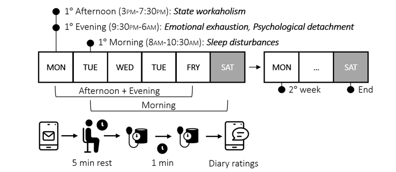
Repeated measures: observations nested within persons
ESM / intensive longitudinal designs
In ESM:
- Level 2 (between): stable differences across persons (“trait-like”)
- Level 1 (within): momentary fluctuations within a person (“state-like”)
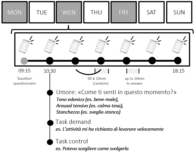
See (Menghini et al., 2023)
Multiple-factor MCFA (compare structures)
Some constructs show different dimensionality within vs between.
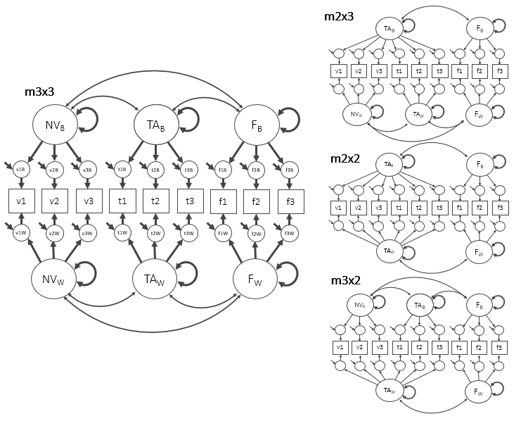
Simulate a 3-factor MCFA dataset (NV, TA, FA)
We simulate 9 ordinal items (3 per factor), repeated within persons.
n_id <- 139
n_rep <- 21
N <- n_id * n_rep
ID <- rep(sprintf("S%03d", 1:n_id), each = n_rep)

# between factors (person-level)
EtaB <- matrix(rnorm(n_id * 3), ncol = 3)
colnames(EtaB) <- c("NV_b","TA_b","FA_b")
EtaB_long <- EtaB[match(ID, sprintf("S%03d", 1:n_id)), ]

# within factors (occasion-level)
EtaW <- matrix(rnorm(N * 3), ncol = 3)
colnames(EtaW) <- c("NV_w","TA_w","FA_w")

lam <- c(0.80, 0.70, 0.75)

make_items <- function(f_w, f_b, prefix) {
  out <- sapply(1:3, function(j) lam[j] * (f_w + f_b) + rnorm(N, 0, 0.9))
  colnames(out) <- paste0(prefix, 1:3)
  out
}

V <- make_items(EtaW[,"NV_w"], EtaB_long[,"NV_b"], "v")
T <- make_items(EtaW[,"TA_w"], EtaB_long[,"TA_b"], "t")
F <- make_items(EtaW[,"FA_w"], EtaB_long[,"FA_b"], "f")

ESM3 <- data.frame(
  ID = ID,
  v1 = cut_likert(V[,1]), v2 = cut_likert(V[,2]), v3 = cut_likert(V[,3]),
  t1 = cut_likert(T[,1]), t2 = cut_likert(T[,2]), t3 = cut_likert(T[,3]),
  f1 = cut_likert(F[,1]), f2 = cut_likert(F[,2]), f3 = cut_likert(F[,3])
)
head(ESM3, 4)
ID v1 v2 v3 t1 t2 t3 f1 f2 f3
1 S001 2 2 4 1 4 3 2 4 5
2 S001 3 2 4 4 3 2 5 2 4
3 S001 5 2 3 2 1 1 5 5 5
4 S001 2 1 1 2 2 2 3 5 5Specify alternative structures
m3x3 <- '
  level: 1
    NV_w =~ v1 + v2 + v3
    TA_w =~ t1 + t2 + t3
    FA_w =~ f1 + f2 + f3
  level: 2
    NV_b =~ v1 + v2 + v3
    TA_b =~ t1 + t2 + t3
    FA_b =~ f1 + f2 + f3
'

m2x3 <- '
  level: 1
    NV_w =~ v1 + v2 + v3
    TA_w =~ t1 + t2 + t3
    FA_w =~ f1 + f2 + f3
  level: 2
    NV_b =~ v1 + v2 + v3 + t1 + t2 + t3
    FA_b =~ f1 + f2 + f3
'Fit and compare
fit2x2 <- cfa(m2x2, ESM3, cluster = "ID", estimator = "MLR")
fit3x2 <- cfa(m3x2, ESM3, cluster = "ID", estimator = "MLR")
fit2x3 <- cfa(m2x3, ESM3, cluster = "ID", estimator = "MLR")
fit3x3 <- cfa(m3x3, ESM3, cluster = "ID", estimator = "MLR")

f2 <- c("df","rmsea.robust","cfi.robust","srmr_within","srmr_between")
round(rbind(
  `2x2` = lavInspect(fit2x2,"fit")[f2],
  `3x2` = lavInspect(fit3x2,"fit")[f2],
  `2x3` = lavInspect(fit2x3,"fit")[f2],
  `3x3` = lavInspect(fit3x3,"fit")[f2]
), 3)
df rmsea.robust cfi.robust srmr_within srmr_between
2x2 52 0.100 0.682 0.094 0.257
3x2 50 0.081 0.802 0.094 0.020
2x3 50 0.060 0.891 0.012 0.257
3x3 48 0.000 1.000 0.012 0.020Negative Level-2 variances (Heywood cases)
Negative residual variances at Level 2 are common in MCFA because:
- error tends to accumulate at Level 1
- Level-2 loadings can be very strong → residual variances close to 0
- sampling fluctuations around ~0 can produce negative estimates
    lhs op  rhs block level    est    se      z pvalue ci.lower ci.upper
22 NV_w ~~ TA_w     1     1  0.003 0.017  0.202  0.840   -0.030    0.037
23 NV_w ~~ FA_w     1     1 -0.013 0.017 -0.772  0.440   -0.047    0.020
24 TA_w ~~ FA_w     1     1 -0.016 0.017 -0.942  0.346   -0.050    0.017
46   v1 ~~   v1     2     2 -0.016 0.008 -2.001  0.045   -0.032    0.000
47   v2 ~~   v2     2     2  0.007 0.009  0.827  0.408   -0.010    0.024
48   v3 ~~   v3     2     2  0.011 0.008  1.420  0.156   -0.004    0.027
49   t1 ~~   t1     2     2  0.007 0.009  0.730  0.465   -0.011    0.025
50   t2 ~~   t2     2     2 -0.013 0.008 -1.654  0.098   -0.028    0.002
51   t3 ~~   t3     2     2 -0.002 0.008 -0.216  0.829   -0.017    0.014
52   f1 ~~   f1     2     2  0.002 0.008  0.294  0.769   -0.013    0.018
53   f2 ~~   f2     2     2 -0.005 0.007 -0.630  0.529   -0.019    0.010
54   f3 ~~   f3     2     2 -0.007 0.008 -0.979  0.328   -0.022    0.007
58 NV_b ~~ TA_b     2     2 -0.034 0.057 -0.596  0.551   -0.145    0.077
59 NV_b ~~ FA_b     2     2 -0.013 0.054 -0.248  0.804   -0.120    0.093
60 TA_b ~~ FA_b 2 2 -0.030 0.051 -0.598 0.550 -0.130 0.069Negative variances and influential-case analysis
If misspecification is unlikely, one pragmatic strategy is influential-case analysis:
- remove clusters (persons) that drive the improper solution
- refit until the negative variance becomes ~0
- compare substantive conclusions
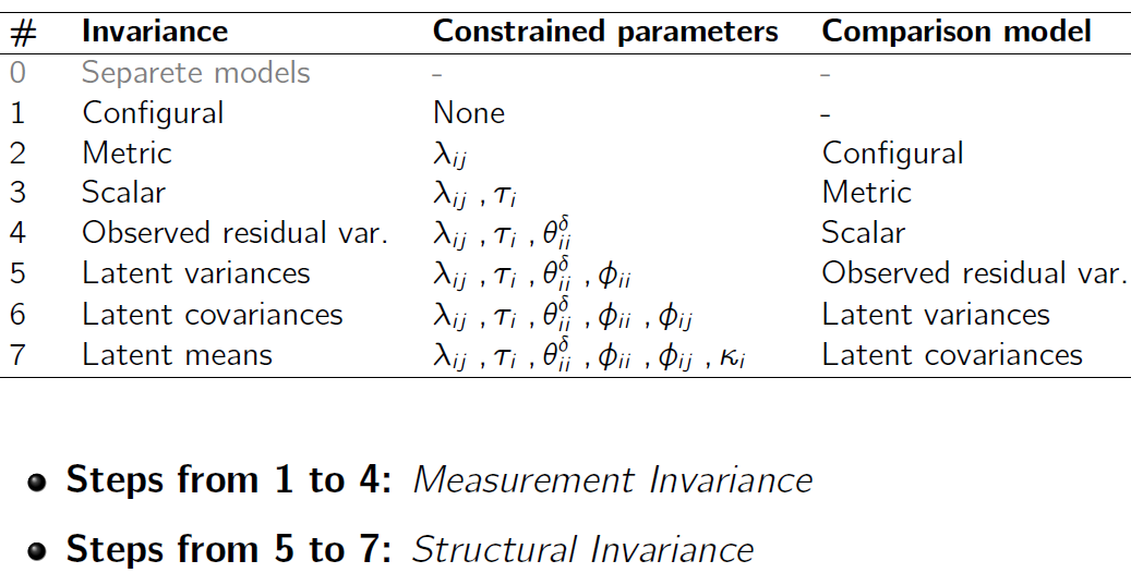
Invariance across levels
Invariance across groups (reminder)
Question: are we measuring the same construct across groups?
Typical approach: multi-group CFA with a sequence of constraints (configural → metric → scalar → …).
Invariance across clusters!?
Multi-group CFA becomes impractical with many clusters (e.g., 139 persons).
Multilevel logic: treat clusters as random effects and focus on cross-level invariance.
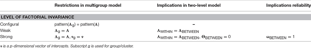
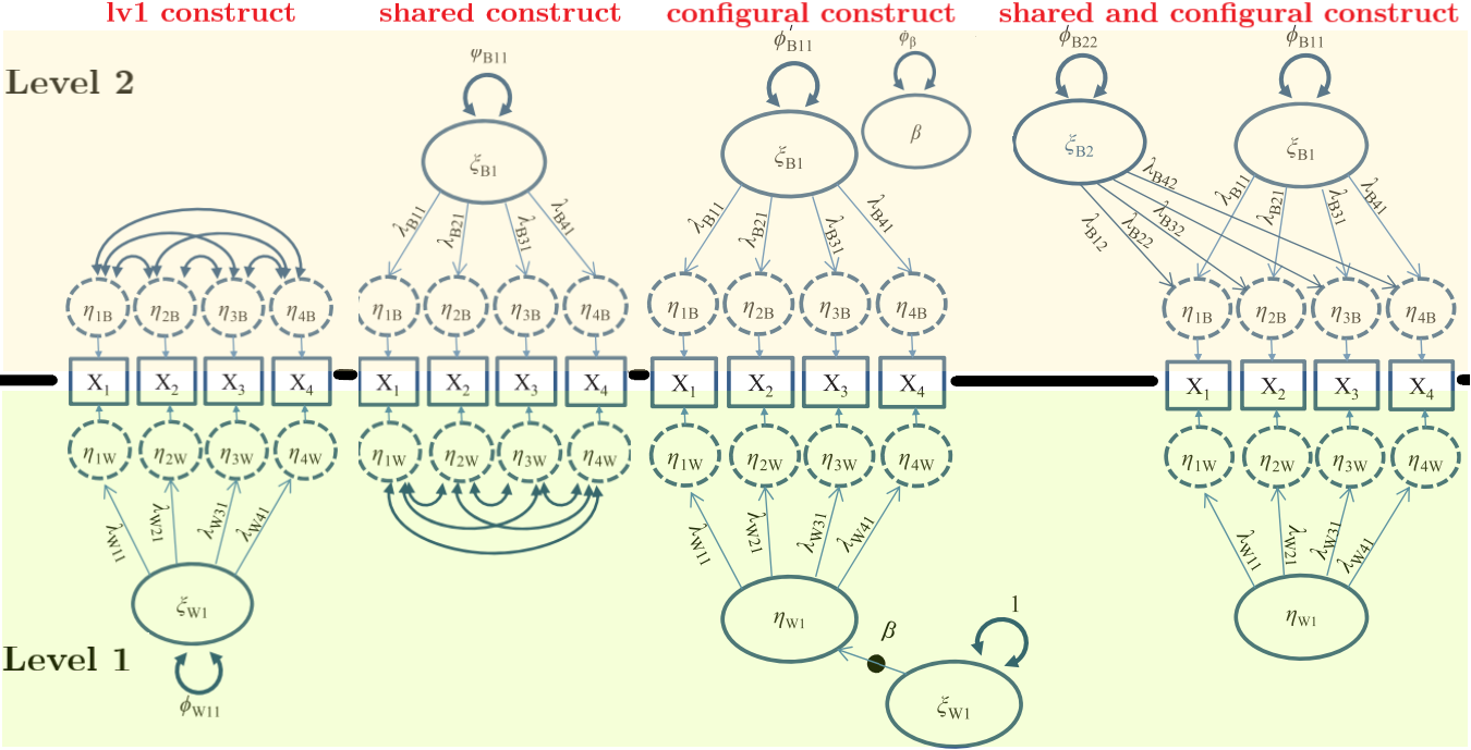
Cross-level invariance: configural
Same factor structure at both levels.
Cross-level invariance: weak (equal loadings)
Same structure + equal (unstandardized) loadings across levels.
Cross-level invariance: “strong”
With psychological data, this is rarely realistic. Treat it as a theoretical benchmark, not a default.
Compare invariance models
fit.conf   <- cfa(conf,   ESM3, cluster = "ID", estimator = "MLR")
fit.weak   <- cfa(weak,   ESM3, cluster = "ID", estimator = "MLR")
fit.strong <- cfa(strong, ESM3, cluster = "ID", estimator = "MLR")

round(rbind(
  conf   = lavInspect(fit.conf,   "fit")[f2],
  weak   = lavInspect(fit.weak,   "fit")[f2],
  strong = lavInspect(fit.strong, "fit")[f2]
), 3)
df rmsea.robust cfi.robust srmr_within srmr_between
conf 48 0 1 0.012 0.020
weak 54 0 1 0.013 0.019
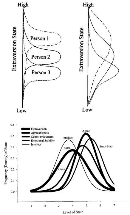
strong 63 0 1 0.013 0.020Multilevel constructs and cross-level invariance
Cross-level invariance is not only “fit”—it’s about construct meaning.
Traits as distributions of states
Some theories treat traits as distributions of states.
This implicitly assumes at least weak cross-level invariance.
Example: state workaholism (simulated)
Luca’s real-data example (slides)
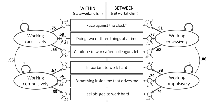
Simulate ESM workaholism (2 factors, 6 items)
n_id <- 135
n_rep <- 30
N <- n_id * n_rep
ID <- rep(sprintf("P%03d", 1:n_id), each = n_rep)
# Between factors
WE_b <- rnorm(n_id, 0, 0.6)
WC_b <- rnorm(n_id, 0, 0.6)
WE_b_long <- rep(WE_b, each = n_rep)
WC_b_long <- rep(WC_b, each = n_rep)
# Within factors
WE_w <- rnorm(N, 0, 1.0)
WC_w <- rnorm(N, 0, 1.0)
# Loadings within
lam_WE_w <- c(0.8, 0.7, 0.75)   # items 1,3,5
lam_WC_w <- c(0.75, 0.70, 0.65) # items 2,4,6
# Loadings between (slight violation on item1)
lam_WE_b <- c(0.60, 0.70, 0.75)
lam_WC_b <- lam_WC_w

WH1 <- lam_WE_w[1]*WE_w + lam_WE_b[1]*WE_b_long + rnorm(N, 0, 0.9)
WH3 <- lam_WE_w[2]*WE_w + lam_WE_b[2]*WE_b_long + rnorm(N, 0, 0.9)
WH5 <- lam_WE_w[3]*WE_w + lam_WE_b[3]*WE_b_long + rnorm(N, 0, 0.9)

WH2 <- lam_WC_w[1]*WC_w + lam_WC_b[1]*WC_b_long + rnorm(N, 0, 0.9)
WH4 <- lam_WC_w[2]*WC_w + lam_WC_b[2]*WC_b_long + rnorm(N, 0, 0.9)
WH6 <- lam_WC_w[3]*WC_w + lam_WC_b[3]*WC_b_long + rnorm(N, 0, 0.9)

dat_wh <- data.frame(
  ID = ID,
  WHLSM1 = cut_likert(WH1),
  WHLSM2 = cut_likert(WH2),
  WHLSM3 = cut_likert(WH3),
  WHLSM4 = cut_likert(WH4),
  WHLSM5 = cut_likert(WH5),
  WHLSM6 = cut_likert(WH6)
)
head(dat_wh, 4)
ID WHLSM1 WHLSM2 WHLSM3 WHLSM4 WHLSM5 WHLSM6
1 P001 1 4 2 5 1 4
2 P001 1 5 1 5 1 4
3 P001 2 4 1 5 1 4
4 P001 4 1 1 4 1 2Cross-level invariance: configural vs weak
conf_wh <- '
  level: 1
    sWE =~ WHLSM1 + WHLSM3 + WHLSM5
    sWC =~ WHLSM2 + WHLSM4 + WHLSM6
  level: 2
    tWE =~ WHLSM1 + WHLSM3 + WHLSM5
    tWC =~ WHLSM2 + WHLSM4 + WHLSM6
'

weak_wh <- '
  level: 1
    sWE =~ a*WHLSM1 + b*WHLSM3 + c*WHLSM5
    sWC =~ d*WHLSM2 + e*WHLSM4 + f*WHLSM6
  level: 2
    tWE =~ a*WHLSM1 + b*WHLSM3 + c*WHLSM5
    tWC =~ d*WHLSM2 + e*WHLSM4 + f*WHLSM6
'

fit.conf_wh <- cfa(conf_wh, dat_wh, cluster = "ID", estimator = "MLR")
fit.weak_wh <- cfa(weak_wh, dat_wh, cluster = "ID", estimator = "MLR")

round(rbind(
  conf = lavInspect(fit.conf_wh, "fit")[c("df","rmsea.robust","cfi.robust","srmr_within","srmr_between")],
  weak = lavInspect(fit.weak_wh, "fit")[c("df","rmsea.robust","cfi.robust","srmr_within","srmr_between")]
), 3)
df rmsea.robust cfi.robust srmr_within srmr_between
conf 16 0.014 0.996 0.014 0.046
weak 20 0.018 0.992 0.015 0.046Partial invariance?
Use modification indices to find which equality constraint is most problematic.
mi <- modificationIndices(fit.weak_wh)
mi[order(mi$mi, decreasing = TRUE), ][1:6, c("lhs","op","rhs","mi")]
lhs op rhs mi
83 WHLSM3 ~~ WHLSM5 18.185
62 WHLSM3 ~~ WHLSM5 17.976
1 sWE =~ WHLSM1 17.796
24 tWE =~ WHLSM1 17.795
53 sWE =~ WHLSM6 10.478
82 WHLSM1 ~~ WHLSM6 6.599Then free one loading across levels (partial weak invariance):
Cross-level homology
Beyond invariance: homology
If cross-level invariance holds (conceptually and empirically), we can test whether the construct has a similar nomological network across levels (cross-level homology).
Take-home: 3 things
- With clustered/repeated data, always think within vs between (two covariance structures).
- In MCFA, global fit can hide L2 misspecification — check SRMR_between.
- Cross-level invariance connects estimation constraints to construct interpretation (trait/state, aggregation, homology).
Exercises → Lab 10
Go to: labs/lab10_multilevel_robustse_twolevelcfa.qmd link
- fit a two-level CFA with
level:+cluster= - compare alternative within/between structures and interpret SRMR
- diagnose (potential) Heywood cases at Level 2
- test (optional) cross-level invariance and partial invariance
Acknowledgments
Thanks AGAIN to Luca Menghini for his slides!
Tip
If you really need anything about multilevel SEM ask Luca!