Specific factors beyond broad constructs

Distinctiveness, interpretability, and predictive validity

Why this extra?

Many papers claim a specific factor or subscale is meaningful simply because a multidimensional model fits.
But once a broader factor exists, the real question becomes:

Is the narrow factor still interpretable and useful after the broad/common variance is modeled?

This deck focuses on that neglected question.

Warning

This deck of slides possibly invalidates many specific findings in the literature. BUT not being able to validate/measure a construct reliably, does not mean your theory is wrong, don’t worry…you just can’t test or study it.

Learning objectives

By the end, students should be able to:

distinguish broad-factor validity from specific-factor validity
explain why fit alone does not justify subscale interpretation
compare correlated-factor, higher-order, bifactor, and bifactor(S-1) logic
evaluate whether a specific factor is well-defined, reliable/determinate, and predictively useful
avoid overstated claims from residualized or observed-score analyses

The motivating problem

Examples you will see in applied work:

anxiety vs math anxiety
intelligence vs executive functions
neuroticism vs depression
general psychopathology vs specific symptom dimensions
general vs domain-specific self-efficacy
mindset vs domain-specific mindset

These are not just “more factors”.

They are claims that a narrow construct remains meaningful (identifiable) once broader variance is present.

A useful reframe

Instead of asking:

“Does the subscale exist?”

Ask three separate questions:

Structural distinctiveness
Is there evidence for separable narrow variance once the broad factor is modeled?
Interpretability
Is that narrow factor well-defined enough to discuss substantively?
Criterion validity
Does it predict anything important above the broad factor?

Note

We’ll see that above the broad factor is not such an easy question to tackle, if you really want to tackle it.

Running example

Does math anxiety predict math performance above general anxiety?

That single sentence hides several different models and several different validity claims.

We need to ask:

Is math anxiety psychometrically separable from general anxiety?
Is the “specific” part reliable or mostly leftover noise?
Does prediction survive latent modeling?
Is the conclusion robust across plausible models?

What usually goes wrong

Common shortcut

Fit a CFA with several related factors
Note that the model fits “well enough”
Use subscale scores in regression
Claim “incremental validity”

The problem

That workflow often confuses:

correlated constructs
residualized variance
measurement error
predictive utility
practical utility

Fit != truth

A model can fit well and still fail the question that matters here:

Is the specific factor interpretable and worth using?

For this topic, always separate:

global fit (CFI/TLI/RMSEA/SRMR)
local diagnostics (residuals, strain, improper estimates)
factor quality (loadings, determinacy, H, omega-type indices)
criterion usefulness (effect sizes, uncertainty, robustness, practical gain)

Four common model families

1. Correlated first-order factors

Broad overlap is represented through factor correlations.

2. Higher-order model

A broad factor explains the correlations among first-order factors.

3. Symmetrical bifactor model

All items load on a general factor and on one group factor.

4. Bifactor(S-1)

A theoretically chosen reference domain defines the general factor; other domains become specific residual factors.

Conceptual map

Model	Broad variance	Narrow variance	Typical attraction	Main danger
Correlated factors	factor correlations	first-order factors	simple, familiar	“unique” meaning may be overstated
Higher-order	higher-order factor	first-order residualized on higher-order	broad vs domains	first-order meaning changes after higher-order layer
Bifactor	general factor on all items	orthogonal group factors	direct separation of common vs specific	overinterpretation, instability, identifiability problems
Bifactor(S-1)	reference-domain-defined general factor	residual domains	often more interpretable	requires strong theory and explicit reference choice

What would count as evidence for a specific factor?

A defensible specific factor usually needs all of the following:

plausible theory for why narrow variance should remain after common variance is modeled
a model that also models the general factor in which the specific factor is statistically admissible and meaningfully defined
adequate factor quality (not just significant loadings)
criterion relations that are stable and not artifacts of scoring/measurement error
reporting that makes clear what the factor means in that parameterization

The key warning

A “specific factor” is often residualized variance.

That can be scientifically meaningful.
But it can also be:

method variance
wording variance
nuisance variance
instability created by a difficult parameterization
a narrow remainder with weak reliability

So the substantive question is not “is it significant?”
It is “what does this remainder represent?”

Observed-score incremental validity is especially risky

A common workflow is:

lm(outcome ~ broad_score + narrow_score, data = dat)

This looks intuitive, but it can be misleading when:

both predictors contain measurement error
they are strongly correlated
“controlling for” one construct changes the meaning of the other
“controlling for” is not what you are really doing

Important

All specific factors are strongly correlated with general factors and share common variance that can be explained by the broader factor.

Why SEM helps

Latent-variable models can help because they allow you to:

model measurement error explicitly
define what “broad” and “specific” mean
compare alternative structures
test criterion relations at the latent level
inspect instability/improper solutions directly
really “control for” the broader factor

But SEM does not magically solve poor theory or weak indicators.

A minimal decision sequence

Start with theory
Fit defensible measurement models (these should already model both factors)
Compare broad+narrow representations
Check local admissibility
Inspect factor quality
Only then test criterion relations
Assess robustness and practical value
Report cautiously

Suggested reporting language

Prefer:

“The residual narrow factor showed limited support and should be interpreted cautiously.”

“After modeling the broad factor, the specific factor retained interpretable variance and showed a modest latent association with the criterion.”

Avoid:

“The subscale demonstrated clear unique validity.”

unless the evidence is unusually strong and consistent.

Code & Simulation

Live coding setup

library(lavaan)
library(semTools)
library(dplyr)
library(ggplot2)

set.seed(1234)
N = 1000

Simulate a broad + narrow factor

# The latent factors (structural truth)
general_anxiety <- rnorm(N)
math_anxiety <- .30*general_anxiety + rnorm(N)
math_performance <- .30*general_anxiety + 0*math_anxiety + rnorm(N)

# Observed items
anx1 = .80*general_anxiety + rnorm(N)
anx2 = .80*general_anxiety + rnorm(N)
anx3 = .80*general_anxiety + rnorm(N)
anx4 = .80*general_anxiety + rnorm(N)
manx1 = .65*general_anxiety + .35*math_anxiety + rnorm(N)
manx2 = .65*general_anxiety + .35*math_anxiety + rnorm(N)
manx3 = .65*general_anxiety + .35*math_anxiety + rnorm(N)
manx4 = .65*general_anxiety + .35*math_anxiety + rnorm(N)

dat <- data.frame(
  anx1,anx2,anx3,anx4,
  manx1,manx2,manx3,manx4,
  math_performance
)
# Sum scores
dat$anxiety <- rowMeans(cbind(anx1,anx2,anx3,anx4))
dat$mat_anx <- rowMeans(cbind(manx1,manx2,manx3,manx4))

Step 1: Factorial validity

‘Classical’ factor analysis

mod_class <- '
  math_anx =~ manx1 + manx2 + manx3 + manx4
'
fit <- cfa(mod_class, data = dat)
fitmeasures(fit, fit.measures = c("cfi","tli","rmsea","srmr"))

  cfi   tli rmsea  srmr 
1.000 1.001 0.000 0.008

parameterestimates(fit,standardized = T)[,c("lhs","op","rhs","est","se","std.lv","std.all")]

       lhs op      rhs   est    se std.lv std.all
1 math_anx =~    manx1 1.000 0.000  0.849   0.642
2 math_anx =~    manx2 0.926 0.065  0.786   0.612
3 math_anx =~    manx3 1.029 0.069  0.873   0.685
4 math_anx =~    manx4 1.001 0.068  0.850   0.653
5    manx1 ~~    manx1 1.028 0.061  1.028   0.588
6    manx2 ~~    manx2 1.031 0.059  1.031   0.625
7    manx3 ~~    manx3 0.863 0.057  0.863   0.531
8    manx4 ~~    manx4 0.970 0.059  0.970   0.573
9 math_anx ~~ math_anx 0.720 0.075  1.000   1.000

We would conclude our measure is valid as it shows perfect fit indices and high and equal loadings across all items

BUT WE ALSO COLLECTED DATA ON ‘ANXIETY’ IN GENERAL…a higher-order factor!

Competing model 1: correlated factors

mod_cf <- '
  math_anx =~ manx1 + manx2 + manx3 + manx4
  gen_anx =~ anx1 + anx2 + anx3 + anx4
  math_anx ~~ gen_anx
'
fit_cf <- sem(mod_cf, data = dat)
fitmeasures(fit_cf, fit.measures = c("cfi","tli","rmsea","srmr"))

  cfi   tli rmsea  srmr 
0.999 0.999 0.011 0.015

parameterestimates(fit_cf,standardized = T)[,c("lhs","op","rhs","est","se","std.lv","std.all")]

        lhs op      rhs   est    se std.lv std.all
1  math_anx =~    manx1 1.000 0.000  0.839   0.635
2  math_anx =~    manx2 0.978 0.061  0.821   0.639
3  math_anx =~    manx3 1.032 0.061  0.865   0.679
4  math_anx =~    manx4 0.992 0.062  0.832   0.640
5   gen_anx =~     anx1 1.000 0.000  0.822   0.646
6   gen_anx =~     anx2 0.927 0.059  0.762   0.618
7   gen_anx =~     anx3 0.994 0.061  0.817   0.643
8   gen_anx =~     anx4 0.906 0.060  0.745   0.586
9  math_anx ~~  gen_anx 0.636 0.049  0.922   0.922
10    manx1 ~~    manx1 1.044 0.055  1.044   0.597
11    manx2 ~~    manx2 0.974 0.052  0.974   0.591
12    manx3 ~~    manx3 0.877 0.049  0.877   0.539
13    manx4 ~~    manx4 1.000 0.053  1.000   0.591
14     anx1 ~~     anx1 0.942 0.051  0.942   0.582
15     anx2 ~~     anx2 0.940 0.049  0.940   0.618
16     anx3 ~~     anx3 0.949 0.051  0.949   0.587
17     anx4 ~~     anx4 1.063 0.054  1.063   0.657
18 math_anx ~~ math_anx 0.704 0.069  1.000   1.000
19  gen_anx ~~  gen_anx 0.676 0.066  1.000   1.000

Competing model 2: higher-order representation

mod_ho <- '
  math_anx =~ manx1 + manx2 + manx3 + manx4
  gen_anx =~ anx1 + anx2 + anx3 + anx4 + math_anx
'
fit_ho <- sem(mod_ho, data = dat)
fitmeasures(fit_ho, fit.measures = c("cfi","tli","rmsea","srmr"))

  cfi   tli rmsea  srmr 
0.999 0.999 0.011 0.015

parameterestimates(fit_ho,standardized = T)[,c("lhs","op","rhs","est","se","std.lv","std.all")]

        lhs op      rhs   est    se std.lv std.all
1  math_anx =~    manx1 1.000 0.000  0.839   0.635
2  math_anx =~    manx2 0.978 0.061  0.821   0.639
3  math_anx =~    manx3 1.032 0.061  0.865   0.679
4  math_anx =~    manx4 0.992 0.062  0.832   0.640
5   gen_anx =~     anx1 1.000 0.000  0.822   0.646
6   gen_anx =~     anx2 0.927 0.059  0.762   0.618
7   gen_anx =~     anx3 0.994 0.061  0.817   0.643
8   gen_anx =~     anx4 0.906 0.060  0.745   0.586
9   gen_anx =~ math_anx 0.941 0.063  0.922   0.922
10    manx1 ~~    manx1 1.044 0.055  1.044   0.597
11    manx2 ~~    manx2 0.974 0.052  0.974   0.591
12    manx3 ~~    manx3 0.877 0.049  0.877   0.539
13    manx4 ~~    manx4 1.000 0.053  1.000   0.591
14     anx1 ~~     anx1 0.942 0.051  0.942   0.582
15     anx2 ~~     anx2 0.940 0.049  0.940   0.618
16     anx3 ~~     anx3 0.949 0.051  0.949   0.587
17     anx4 ~~     anx4 1.063 0.054  1.063   0.657
18 math_anx ~~ math_anx 0.105 0.029  0.149   0.149
19  gen_anx ~~  gen_anx 0.676 0.066  1.000   1.000

Competing model 3: bifactor representation

mod_bi <- '
  math_anx =~ manx1 + manx2 + manx3 + manx4
  gen_anx =~ anx1 + anx2 + anx3 + anx4 + manx1 + manx2 + manx3 + manx4
  
  gen_anx ~~ 0*math_anx
'
fit_bi <- sem(mod_bi, data = dat)
fitmeasures(fit_bi, fit.measures = c("cfi","tli","rmsea","srmr"))

  cfi   tli rmsea  srmr 
1.000 1.000 0.000 0.012

parameterestimates(fit_bi,standardized = T)[,c("lhs","op","rhs","est","se","std.lv","std.all")]

        lhs op      rhs   est    se std.lv std.all
1  math_anx =~    manx1 1.000 0.000  0.352   0.266
2  math_anx =~    manx2 0.467 0.231  0.165   0.128
3  math_anx =~    manx3 1.002 0.328  0.353   0.277
4  math_anx =~    manx4 1.230 0.438  0.433   0.333
5   gen_anx =~     anx1 1.000 0.000  0.824   0.647
6   gen_anx =~     anx2 0.925 0.059  0.762   0.618
7   gen_anx =~     anx3 0.988 0.061  0.814   0.640
8   gen_anx =~     anx4 0.906 0.060  0.746   0.586
9   gen_anx =~    manx1 0.931 0.065  0.767   0.580
10  gen_anx =~    manx2 0.960 0.064  0.791   0.616
11  gen_anx =~    manx3 0.964 0.063  0.794   0.622
12  gen_anx =~    manx4 0.910 0.064  0.749   0.576
13 math_anx ~~  gen_anx 0.000 0.000  0.000   0.000
14    manx1 ~~    manx1 1.036 0.063  1.036   0.593
15    manx2 ~~    manx2 0.995 0.051  0.995   0.604
16    manx3 ~~    manx3 0.871 0.058  0.871   0.536
17    manx4 ~~    manx4 0.943 0.078  0.943   0.557
18     anx1 ~~     anx1 0.940 0.051  0.940   0.581
19     anx2 ~~     anx2 0.940 0.049  0.940   0.618
20     anx3 ~~     anx3 0.954 0.051  0.954   0.590
21     anx4 ~~     anx4 1.061 0.054  1.061   0.656
22 math_anx ~~ math_anx 0.124 0.060  1.000   1.000
23  gen_anx ~~  gen_anx 0.678 0.066  1.000   1.000

What to compare across models

Do not ask only “which model fits best?”

Also compare:

whether parameter estimates are admissible
whether the specific factor has meaningful loadings
whether the narrow factor is determinate/reliable enough
whether conclusions change under plausible reparameterizations

Factor quality matters

For broad vs specific claims, add checks such as:

salient standardized loadings
factor determinacy
construct replicability / (H)
omega-based indices
explained common variance (for bifactor contexts)

A specific factor with low determinacy or weak replicability is hard to interpret, even if global fit looks good.

Optional indices for bifactor models

# After extracting standardized loadings / residual variances,
# inspect indices such as omega hierarchical, omega subscale,
# ECV, PUC, H, and factor determinacy.
library(BifactorIndicesCalculator)
bifactorIndices(fit_bi)

$ModelLevelIndices
   ECV.gen_anx            PUC  Omega.gen_anx OmegaH.gen_anx 
     0.9157073      0.7857143      0.8401305      0.8060378 

$FactorLevelIndices
            ECV_SS     ECV_SG    ECV_GS     Omega    OmegaH         H        FD
math_anx 0.1609079 0.08429275 0.8390921 0.7465064 0.1117941 0.2314392 0.4835506
gen_anx  0.9157073 0.91570725 0.9157073 0.8401305 0.8060378 0.8277219 0.9011336

$ItemLevelIndices
           IECV
manx1 0.8256587
manx2 0.9584576
manx3 0.8347653
manx4 0.7492171
anx1  1.0000000
anx2  1.0000000
anx3  1.0000000
anx4  1.0000000

Step 2 - Criterion validity

‘Classical’ approach

mod_class <- '
  math_anx =~ manx1 + manx2 + manx3 + manx4
  math_performance ~ math_anx
'
fit <- cfa(mod_class, data = dat)

               lhs op      rhs   est    se std.lv std.all
5 math_performance  ~ math_anx 0.342 0.047  0.288   0.272

summary(lm(math_performance~mat_anx,dat))


Call:
lm(formula = math_performance ~ mat_anx, data = dat)

Residuals:
     Min       1Q   Median       3Q      Max 
-3.15021 -0.72446  0.01687  0.70175  3.01907 

Coefficients:
            Estimate Std. Error t value Pr(>|t|)    
(Intercept)  0.02053    0.03263   0.629    0.529    
mat_anx      0.25212    0.03351   7.523 1.19e-13 ***
---
Signif. codes:  0 '***' 0.001 '**' 0.01 '*' 0.05 '.' 0.1 ' ' 1

Residual standard error: 1.032 on 998 degrees of freedom
Multiple R-squared:  0.05366,   Adjusted R-squared:  0.05271 
F-statistic: 56.59 on 1 and 998 DF,  p-value: 1.194e-13

We would conclude our measure is a good predictor of math performance, but is it for real?

…we know from the data generating model that it should not be! Isn’t it?

SEM with correlated factors

mod_cf <- '
  math_anx =~ manx1 + manx2 + manx3 + manx4
  gen_anx =~ anx1 + anx2 + anx3 + anx4
  math_anx ~~ gen_anx
  math_performance ~ math_anx+gen_anx
'
fit_cf <- sem(mod_cf, data = dat)

                lhs op      rhs    est    se std.lv std.all
10 math_performance  ~ math_anx -0.126 0.246 -0.105  -0.100
11 math_performance  ~  gen_anx  0.519 0.254  0.425   0.401

summary(lm(math_performance~mat_anx+anxiety,dat))


Call:
lm(formula = math_performance ~ mat_anx + anxiety, data = dat)

Residuals:
     Min       1Q   Median       3Q      Max 
-3.15389 -0.72012  0.01263  0.71534  2.85762 

Coefficients:
            Estimate Std. Error t value Pr(>|t|)    
(Intercept)  0.02606    0.03230   0.807   0.4199    
mat_anx      0.10840    0.04486   2.416   0.0159 *  
anxiety      0.22371    0.04704   4.756 2.26e-06 ***
---
Signif. codes:  0 '***' 0.001 '**' 0.01 '*' 0.05 '.' 0.1 ' ' 1

Residual standard error: 1.021 on 997 degrees of freedom
Multiple R-squared:  0.07466,   Adjusted R-squared:  0.0728 
F-statistic: 40.22 on 2 and 997 DF,  p-value: < 2.2e-16

What’s going on here? Why do sum scores suggest both factors have an effect?

Bifactor representation

mod_bi <- '
  math_anx =~ manx1 + manx2 + manx3 + manx4
  gen_anx =~ anx1 + anx2 + anx3 + anx4 + manx1 + manx2 + manx3 + manx4
  
  gen_anx ~~ 0*math_anx
  math_performance ~ math_anx+gen_anx
'
fit_bi <- sem(mod_bi, data = dat)

                lhs op      rhs   est    se std.lv std.all
14 math_performance  ~ math_anx 0.064 0.197  0.023   0.022
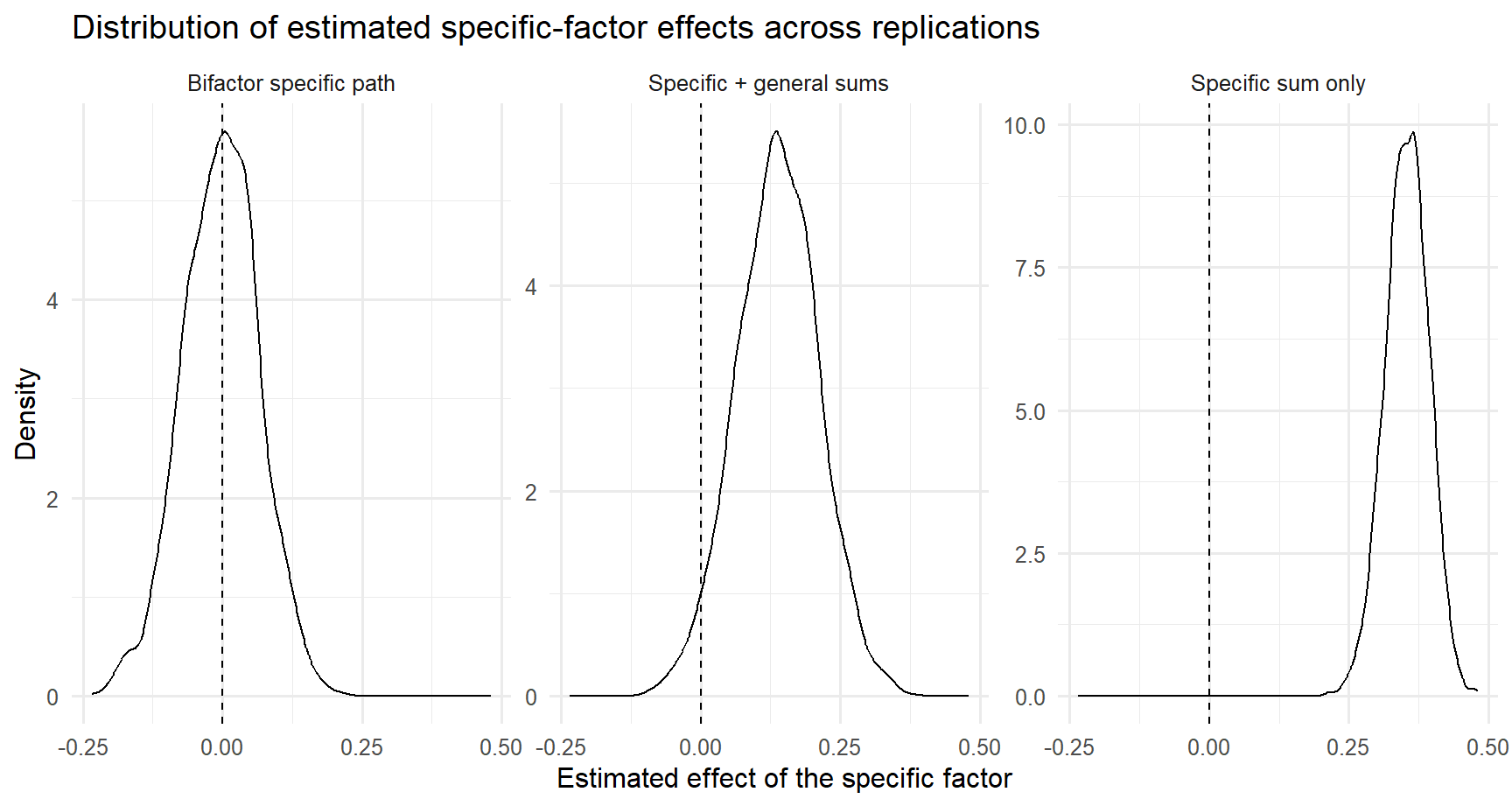
15 math_performance  ~  gen_anx 0.383 0.049  0.314   0.297

Simulation results (bg=.40; bs=0; rgs=.40)

model	mean_estimate	sd_estimate	prop_significant
Bifactor specific path	-0.004	0.068	0.059
Specific + general sums	0.137	0.073	0.452
Specific sum only	0.354	0.039	1.000

Concluding remarks

Implications for non-validation results

Well, everything applies to all contexts. You cannot just control for intelligence using the Raven matrices…you should model intelligence as a general latent factor and test whether your specific executive funtion measures, visuo-spatial abilities, creative skills predict the desired outcome beyond the latent g factor.

This is well known in literature…but we always ignore it (Westfall & Yarkoni, 2016)

A practical rubric

Question	If “no”	Consequence
Is the specific factor theoretically motivated?	weak theory	do not over-interpret
Are estimates admissible and stable?	improper / unstable	stop and rethink model
Is the specific factor well-defined?	weak loadings / low determinacy	avoid strong substantive claims
Does it add latent predictive information?	null / fragile effects	no evidence for unique criterion value
Is the gain practically meaningful?	trivial improvement	probably not worth using

Three take-home messages

Specific factors are not automatically meaningful
Good fit is not enough.
Interpretability comes before prediction claims
First ask whether the factor is well-defined.
Incremental validity must be modeled carefully
Measurement error, parameterization, and out-of-sample performance all matter.

Self-study exercises

Take a scale with a plausible broad+narrow structure from your own area.
Write down what the “specific factor” would mean after broad variance is removed.
Fit at least two plausible measurement models.
Compare not just fit, but the meaning of the narrow factor.
Test one criterion relation.
Ask whether the conclusion is robust across models.
If you use observed scores, add a cross-validated prediction comparison.

What I would report in a paper

Minimum reporting before claiming “specific-factor validity”:

why a broad+narrow representation is theoretically expected
which competing measurement models were tested
global fit + local diagnostics
factor quality indices for the specific factor
the exact criterion model
robustness of the criterion conclusion across plausible specifications
whether the predictive gain is practically meaningful

References

Eid, M., Krumm, S., Koch, T., & Schulze, J. (2018). Bifactor Models for Predicting Criteria by General and Specific Factors: Problems of Nonidentifiability and Alternative Solutions. Journal of Intelligence, 6(3), 42. https://doi.org/10.3390/jintelligence6030042

Rodriguez, A., Reise, S. P., & Haviland, M. G. (2016). Evaluating bifactor models: Calculating and interpreting statistical indices. Psychological Methods, 21(2), 137–150. https://doi.org/10.1037/met0000045

Westfall, J., & Yarkoni, T. (2016). Statistically Controlling for Confounding Constructs Is Harder than You Think. PLOS ONE, 11(3), e0152719. https://doi.org/10.1371/journal.pone.0152719

Specific factors beyond broad constructs

Why this extra?

Learning objectives

The motivating problem

A useful reframe

Running example

What usually goes wrong

Fit != truth

Four common model families

Conceptual map

What would count as evidence for a specific factor?

The key warning

Observed-score incremental validity is especially risky

Why SEM helps

A minimal decision sequence

Suggested reporting language

Code & Simulation

Live coding setup

Simulate a broad + narrow factor

Step 1: Factorial validity

‘Classical’ factor analysis

Competing model 1: correlated factors

Competing model 2: higher-order representation

Competing model 3: bifactor representation

What to compare across models

Factor quality matters

Optional indices for bifactor models

Step 2 - Criterion validity

‘Classical’ approach

SEM with correlated factors

Bifactor representation

Simulation results (bg=.40; bs=0; rgs=.40)

Concluding remarks

Implications for non-validation results

A practical rubric

Three take-home messages

Self-study exercises

What I would report in a paper

Further reading

References