Structural Equation Models

Measurement + structure (capstone)

Tommaso Feraco

Today in the workflow

Specify → Identify → Estimate → Evaluate → Revise/Report

Today: full SEM = measurement model (CFA) + structural model (paths among latent variables).
We will repeat fit/diagnostics on purpose: by now it should become a habit (global + local).

Learning objectives

By the end of this session you should be able to:

• Connect the CFA measurement model to the SEM structural model (two-step mindset)
• Understand how SEM is represented in matrices (\(Λ\), \(B\), \(Γ\), \(Φ\), \(Ψ\), \(Θ\))
• Fit a full SEM in lavaan and interpret parameters + fit indices + diagnostics
• Compare plausible SEMs (nested comparisons) and justify modifications transparently

Structural equation models

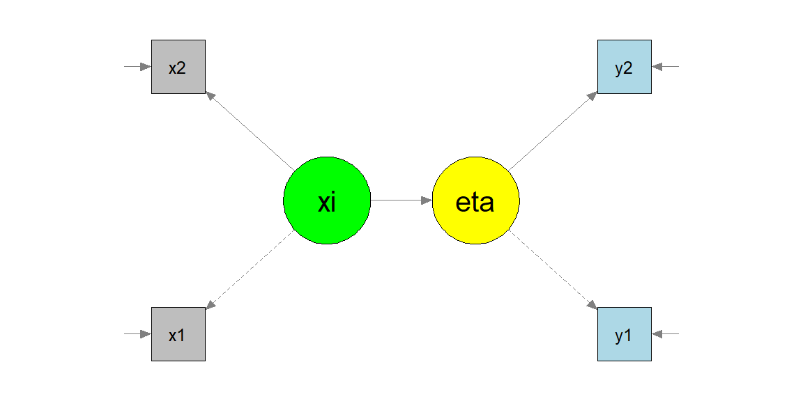
Up to now, we have seen how to model the relationship between different variables/constructs at the same time (path analysis) and how to build a measurement model with one or more latent variables.

A complete SEM takes both of these things and put them together.

The two parts of a SEM

• The measurement model

  • \(x = \Lambda_x\xi + \delta\)

  • \(y = \Lambda_y\eta + \epsilon\)

• The structural model

  • \(\eta = B\eta + \Gamma\xi + \zeta\)

already seen in the first slides

Matrices

These models (can) have all the possible matrices:

• Loadings and coefficients matrices

  • \(\Lambda^x\) - relation among \(\xi\) and \(x\)
  • \(\Lambda^y\) - relation among \(\eta\) and \(y\)
  • \(B\) - relation among \(\eta\) and \(\eta\)
  • \(\Gamma\) - relation among \(\xi\) and \(\eta\)

• Covariance matrices

  • \(\Theta^\delta\) - \(x\) errors
  • \(\Theta^\epsilon\) - \(y\) errors
  • \(\Psi\) - \(\eta\) errors
  • \(\Phi\) - relations among \(\eta\)

Different models are allowed based on the way we define relationships among variables

… lavaan matrices

lavaan does not distinguish between endogenous and exogenous variables. This leads to an easier parametrization and to four matrices only:

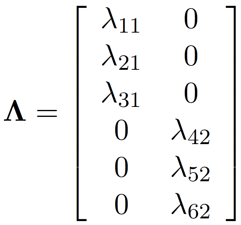
• \(\Lambda\) factor loadings matrix \([p x m]\)
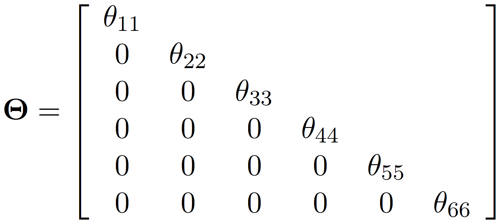
• \(\Theta\) measurement residual errors covariance matrix \([p x p]\)
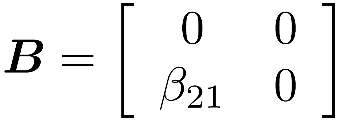
• \(B\) regression coefficients matrix \([m x m]\)
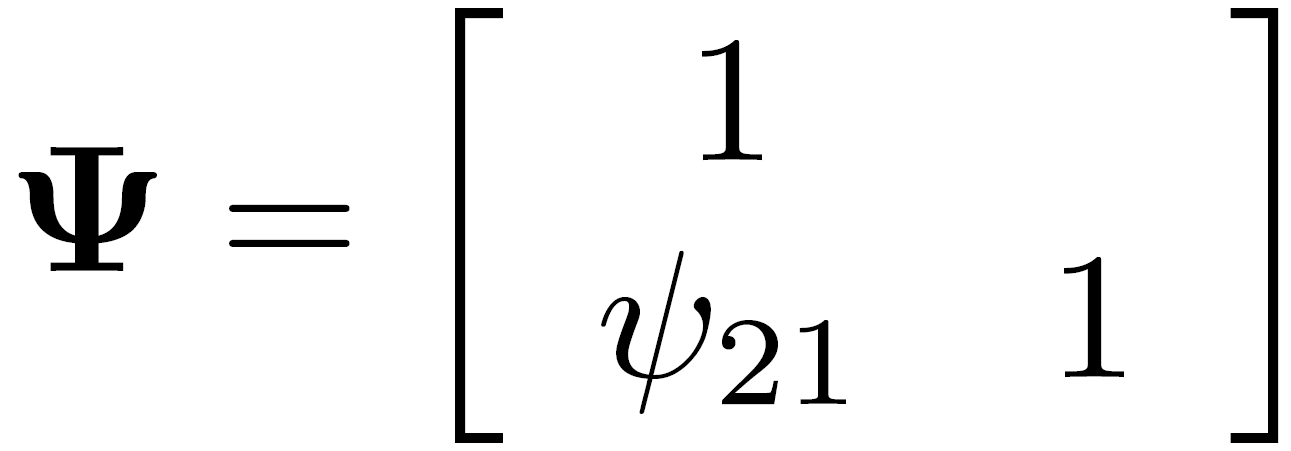
• \(\Psi\) residual structural errors covariance matrix \([m x m]\)

With p being the number of manifest variables and m being the number of latent variables.

The lavaan matrices

Lambda: matrix of loadings

Beta: regression coefficients

Psi: residual structural errors matrix

Theta: observed variance-covariance matrix

A SEM example - simulation

library(lavaan)
dSEM <- simulateData("xi =~ .74*x1 + .65*x2 # note the =~
                      eta =~ .56*y1 + .75*y2
                      eta ~ .30*xi # and the ~ only
                     ", sample.nobs = 1000)

A SEM example - specification and constraints

fit <- sem(model = "xi =~ x1 + x2
                     eta =~ y1 + y2
                     eta ~ xi", data = dSEM)

Constraints

To estimate the model we need to set constraints:

• the sem or cfa functions default is setting to 1 one loading for each latent variable
• an alternative is to standardized latent variables using the std.lv = TRUE option

Constraints: default

[...]
Latent Variables:
                   Estimate  Std.Err  z-value  P(>|z|)   Std.lv  Std.all
  xi =~                                                                 
    x1                1.000                               0.606    0.493
    x2                1.164    0.542    2.146    0.032    0.706    0.589
  eta =~                                                                
    y1                1.000                               0.488    0.435
    y2                1.692    0.868    1.949    0.051    0.825    0.656

[...]
Variances:
                   Estimate  Std.Err  z-value  P(>|z|)   Std.lv  Std.all
   .x1                1.147    0.179    6.402    0.000    1.147    0.757
   .x2                0.938    0.236    3.972    0.000    0.938    0.653
   .y1                1.018    0.130    7.821    0.000    1.018    0.811
   .y2                0.900    0.352    2.559    0.011    0.900    0.569
    xi                0.368    0.177    2.074    0.038    1.000    1.000
   .eta               0.227    0.118    1.923    0.055    0.954    0.954

[...]

Constraints: std.lv=T

[...]
Latent Variables:
                   Estimate  Std.Err  z-value  P(>|z|)   Std.lv  Std.all
  xi =~                                                                 
    x1                0.606    0.146    4.148    0.000    0.606    0.493
    x2                0.706    0.168    4.193    0.000    0.706    0.589
  eta =~                                                                
    y1                0.476    0.124    3.845    0.000    0.488    0.435
    y2                0.806    0.215    3.746    0.000    0.825    0.656

[...]
Variances:
                   Estimate  Std.Err  z-value  P(>|z|)   Std.lv  Std.all
   .x1                1.147    0.179    6.402    0.000    1.147    0.757
   .x2                0.938    0.236    3.972    0.000    0.938    0.653
   .y1                1.018    0.130    7.821    0.000    1.018    0.811
   .y2                0.900    0.352    2.559    0.011    0.900    0.569
    xi                1.000                               1.000    1.000
   .eta               1.000                               0.954    0.954

[...]

lavaan matrices

inspect(fit, "std") # OR "est"

$lambda
      xi   eta
x1 0.493 0.000
x2 0.589 0.000
y1 0.000 0.435
y2 0.000 0.656

$theta
      x1    x2    y1    y2
x1 0.757                  
x2 0.000 0.653            
y1 0.000 0.000 0.811      
y2 0.000 0.000 0.000 0.569

$psi
       xi   eta
xi  1.000      
eta 0.000 0.954

$beta
       xi eta
xi  0.000   0
eta 0.215   0

SEM identification

Once again, remember that identification is a topic relevant to all structural equation models.

If an unknown parameter in \(\theta\) can be written as a function of one or more elements of \(\Sigma\), that parameter is identified.

If all unknown parameters in \(\theta\) are identified, the model is identified.

• the t-rule (again)
• the Two-Steps rule

Two-Steps rule

• Step 1. Treat the model as a confirmatory factor analysis: view the original \(x\) and \(y\) as \(x\) variables and the original \(\xi\) and \(\eta\) as \(\xi\) variables. The only relationship between latent variables of interest are their variance and covariance \(Phi\). That is, ignore the \(B\), \(\Gamma\), and \(\Psi\) elements.

  \(\rightarrow\) apply CFA identification rules

• Step 2. Examine the latent variable equation of the original model (\(\eta = B\eta + \Gamma\xi + \zeta\)), assuming that each latent variable is an observed variable that is perfectly measured.

Two-Steps rule

Summary

If the first step shows that the measurement parameters are identified and the second step shows that the latent variable model parameters also are identified, then this is suficient to identify the whole model.

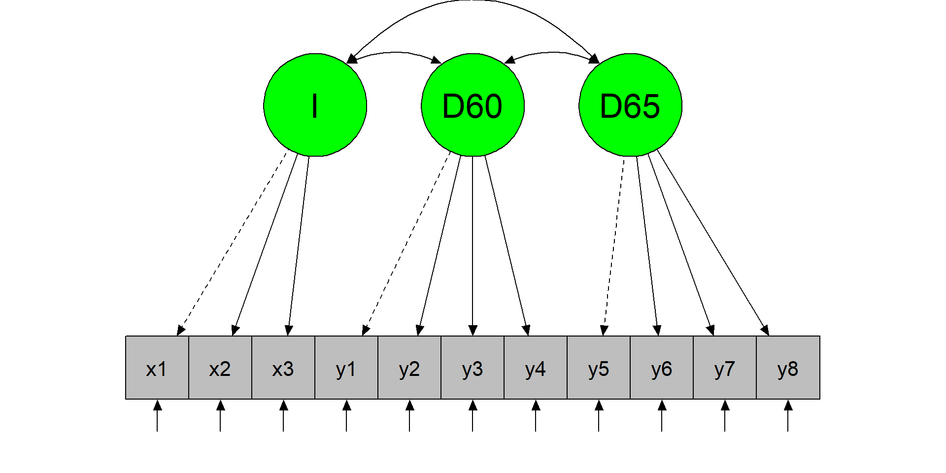
Political democracy dataset

Bollen (1989) studied the relation between industrialization in 1960 and political democracy of developing countries in 1960 and 1965.

We have 11 variables

    y1  y2    y3  y4   y5   y6    y7   y8   x1   x2   x3
1 2.50 0.0  3.33 0.0 1.25 0.00  3.73 3.33 4.44 3.64 2.56
2 1.25 0.0  3.33 0.0 6.25 1.10  6.67 0.74 5.38 5.06 3.57
3 7.50 8.8 10.00 9.2 8.75 8.09 10.00 8.21 5.96 6.26 5.22

A first latent variable, Industrialization (\(I = x_1 + x_2 + x_3\))

A second latent variable, political democracy in 1960 (\(D60 = y_1 + y_2 + y_3 + y_4\))

A third latent variable, political democracy in 1965 (\(D65 = y_5 + y_6 + y_7 + y_8\)).

LET'S APLLY THE TWO-STEPS RULE

Step 1 - model plot

The CFA model

Step 1 - model specification and results

The CFA model

m <- "I =~ x1 + x2 + x3
D60 =~ y1 + y2 + y3 + y4
D65 =~ y5 + y6 + y7 + y8
"

fit1 <- sem(m, data = PoliticalDemocracy)
fit1@Fit@converged

[1] TRUE

PARAMETERS ARE ALL IDENTIFIED. LET'S GO TO STEP 2

Step 2 - model plot

The structural model

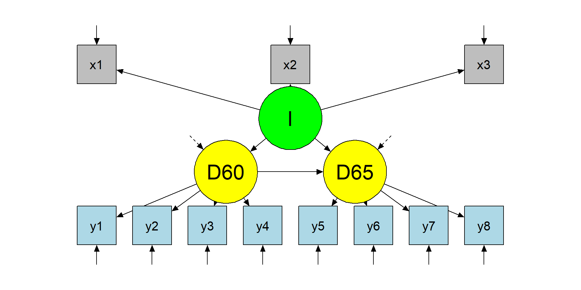
Step 2 - model specification and results

The structural model

m2 <- "I =~ x1 + x2 + x3
D60 =~ y1 + y2 + y3 + y4
D65 =~ y5 + y6 + y7 + y8
D65 ~ I + D60
D60 ~ I
"

fit2 <- sem(m2, data = PoliticalDemocracy)
fit2@Fit@converged

[1] TRUE

STRUCTURAL PARAMETERS ARE ALSO IDENTIFIED.

LET'S DEFINE THE MODEL CONSIDERING LONGITUDINAL MEASURES

Final model

The modified model

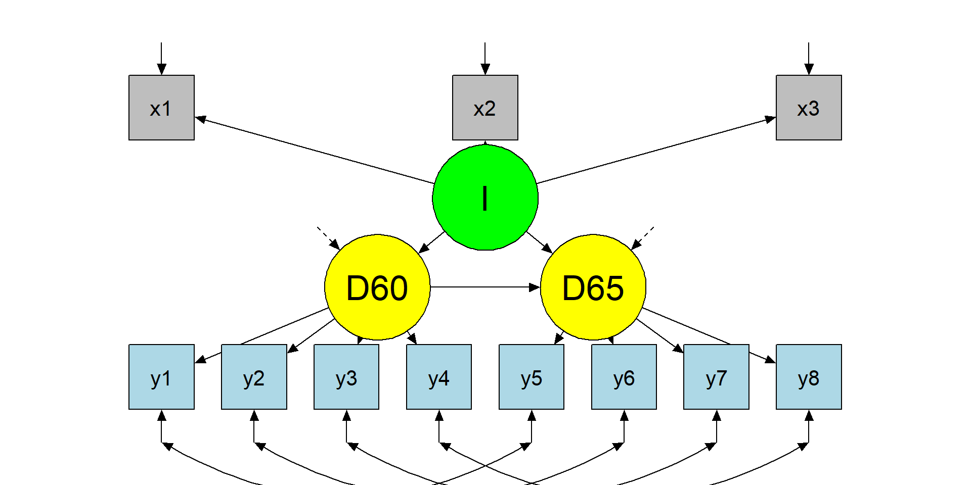
Final model specification

The modified model

m3 <- "I =~ x1 + x2 + x3
D60 =~ y1 + y2 + y3 + y4
D65 =~ y5 + y6 + y7 + y8
D65 ~ I + D60
D60 ~ I
y1 ~~ y5
y2 ~~ y6
y3 ~~ y7
y4 ~~ y8
"

SAME ITEMS AT DIFFERENT TIME POINTS HAVE CORRELATED RESIDUALS

Final model results

The modified model

(fit3 <- sem(m3, data = PoliticalDemocracy))

lavaan 0.6-19 ended normally after 58 iterations

  Estimator                                         ML
  Optimization method                           NLMINB
  Number of model parameters                        29

  Number of observations                            75

Model Test User Model:
                                                      
  Test statistic                                50.835
  Degrees of freedom                                37
  P-value (Chi-square)                           0.064

inspect(fit3, what = "fitmeasures")[
  c("cfi", "srmr", "rmsea")]

       cfi       srmr      rmsea 
0.97952316 0.05011528 0.07060935 

MODEL FIT IS GOOD!

Model comparisons

anova(fit1,fit2,fit3)

Warning: lavaan->lavTestLRT():  
   some models have the same degrees of freedom

Chi-Squared Difference Test

     Df    AIC    BIC  Chisq Chisq diff   RMSEA Df diff Pr(>Chisq)    
fit3 37 3166.3 3233.5 50.835                                          
fit1 41 3179.9 3237.9 72.462     21.626 0.24239       4  0.0002378 ***
fit2 41 3179.9 3237.9 72.462      0.000 0.00000       0               
---
Signif. codes:  0 '***' 0.001 '**' 0.01 '*' 0.05 '.' 0.1 ' ' 1

Model comparisons

We can also compare the models using fit indices:

	chisq	df	cfi	tli	srmr	rmsea	aic	bic
model1	72.462	41	0.953	0.938	0.055	0.101	3179.918	3237.855
model2	72.462	41	0.953	0.938	0.055	0.101	3179.918	3237.855
model3	50.835	37	0.980	0.970	0.050	0.071	3166.292	3233.499

WHAT IS THE BEST MODEL? QUESTIONS? COMMENTS?

Exercise

The EAT dataset

The dataset includes 13 items that measure ‘peer pressure’, ‘social media use’, ‘social comparison’, and ‘eating disorders’.

load("../data/Exercise4_1.Rdata")
round(head(dE4_1),2)

    PP1   PP2   PP3   PP4   SM1   SM2   SM3   SM4   SC1   SC2   SC3   ED1   ED2
1  0.23  1.91  0.59 -0.70  2.31  1.06  1.43 -0.77  1.18  2.20  0.18 -0.38  1.61
2 -0.65 -3.18 -0.84 -0.43  0.69  0.10  1.24  0.51 -1.87 -1.17 -1.23 -1.74 -1.73
3  0.26 -1.46 -0.43 -0.05 -0.21 -0.46 -0.02  1.26  1.39  1.03  0.90  1.07  2.04
4 -0.68 -0.29 -0.08 -2.24 -0.64  0.47 -0.76  0.58  1.22  0.97  2.73  0.71  0.32
5 -0.06  0.89  0.04 -0.41  0.17  1.02  0.18  0.61  3.74  1.38  1.85  1.25  0.66
6 -0.29 -2.74 -0.52  2.58  0.15 -1.08  1.08  0.99  1.32 -0.24  0.93 -0.97 -0.68

The theoretical model

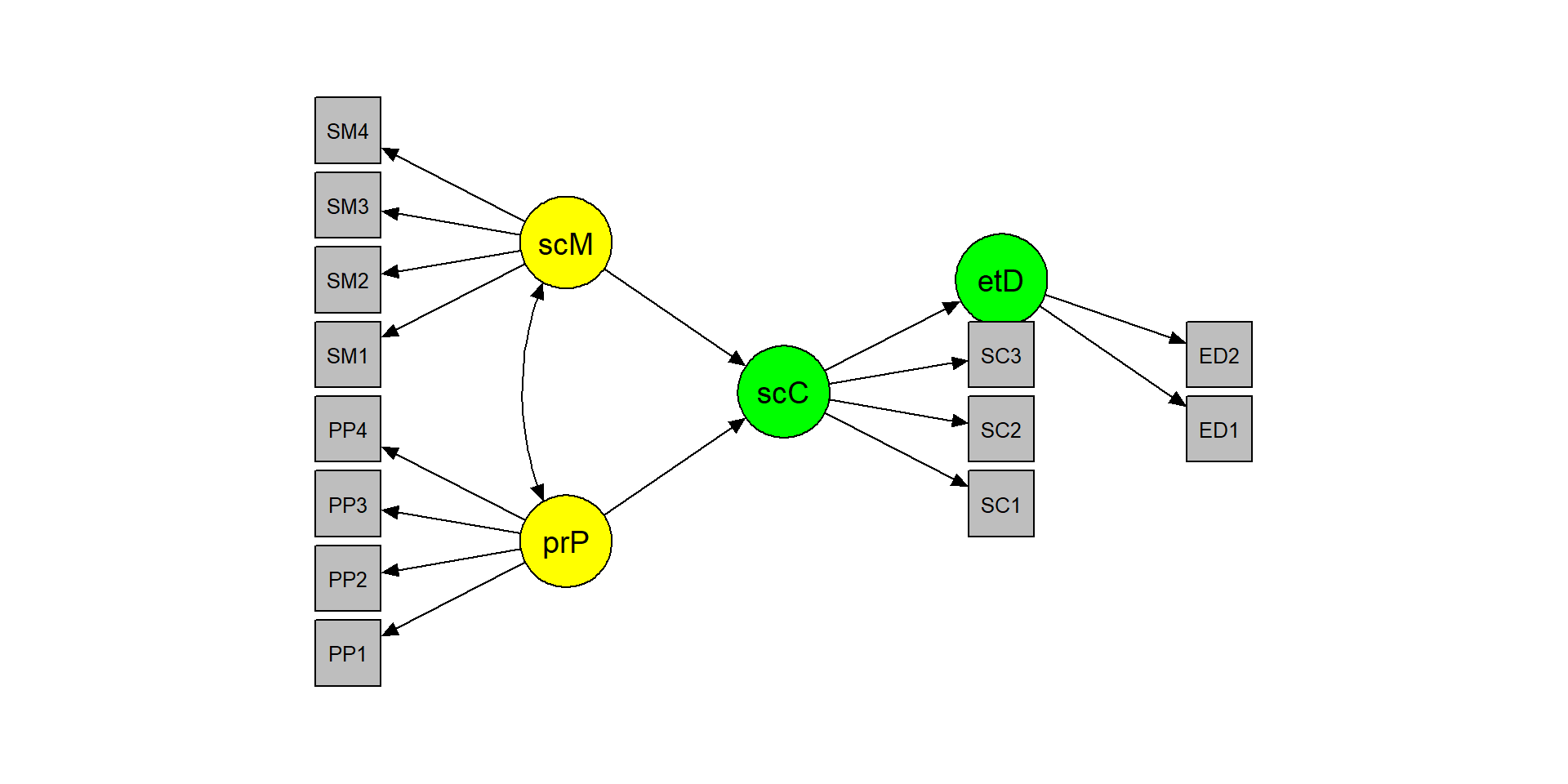
The exercise

1. Apply the two-step rule:
   1. Test the CFA model
   2. Test the structural model
2. Inspect model results and fit indices
   • Are the hypotheses confirmed?
   • Does the model fit the data well?
3. If the model is not satisfactory, understand why and change it
4. Draw the model (in R, ppt, or with a pencil)
5. Try to fit a simple path model using sum scores instead of latent scores

Model specification

STEP 1 and 2

m1 <- "
 # CFA model
 peerPressure =~ PP1 + PP2 + PP3 + PP4
 socialMedia =~ SM1 + SM2 + SM3 + SM4
 socialComparison =~ SC1 + SC2 + SC3
 eatingDisorder =~ ED1 + ED2
"
fit1 <- sem(m1, data = dE4_1, std.lv=T)
fit1@Fit@converged
m2 <- "
 [...]
 # Structural model
 eatingDisorder ~ socialComparison
 socialComparison ~ peerPressure + socialMedia"
fit2 <- sem(m2, data = dE4_1, std.lv=T)
fit2@Fit@converged

OK?

Results and fit

summary(fitE4_1, std=T)

[...]
Regressions:
                     Estimate  Std.Err  z-value  P(>|z|)   Std.lv  Std.all
  eatingDisorder ~                                                        
    socialComparsn      0.344    0.047    7.322    0.000    0.356    0.356
  socialComparison ~                                                      
    peerPressure        0.139    0.038    3.636    0.000    0.125    0.125
    socialMedia         0.455    0.049    9.221    0.000    0.411    0.411

[...]

fitmeasures(fitE4_1, 
            fit.measures = 
            c("cfi", "tli", "srmr", "rmsea"))

  cfi   tli  srmr rmsea 
0.880 0.846 0.044 0.065 

Model modification

modificationIndices(fitE4_1, sort. = T)[1:10,]

                 lhs op rhs      mi    epc sepc.lv sepc.all sepc.nox
120              SM1 ~~ SC2 328.967  0.565   0.565    0.628    0.628
49       socialMedia =~ SC2  56.910  0.378   0.378    0.289    0.289
57  socialComparison =~ SM1  54.668  0.292   0.323    0.283    0.283
121              SM1 ~~ SC3  51.713 -0.235  -0.235   -0.231   -0.231
50       socialMedia =~ SC3  30.539 -0.277  -0.277   -0.206   -0.206
119              SM1 ~~ SC1  22.069 -0.151  -0.151   -0.154   -0.154
143              SC1 ~~ SC3  19.170  0.293   0.293    0.285    0.285
74               PP1 ~~ PP2  18.341  0.665   0.665    1.201    1.201
97               PP3 ~~ PP4  15.333  0.126   0.126    0.109    0.109
58  socialComparison =~ SM2  13.081 -0.146  -0.162   -0.137   -0.137

m2.1 <- "
[...]
# Residual correlations
SM1 ~~ SC2
"
fitmeasures(fit2.1, ...)

  cfi   tli  srmr rmsea 
0.995 0.994 0.023 0.013 

Why sum scores can mislead (measurement error → attenuation)

If an observed score \((X)\) is a noisy measure of a latent variable, measurement error tends to attenuate associations.

A classic intuition (simple linear setting):

\[ \hat\beta_{\text{observed}} \approx \hat\beta_{\text{latent}} \times \rho_{xx} \]

where \((\rho_{xx})\) is reliability of \((X)\).

This is exactly why latent-variable SEM can change “structural” conclusions even when factor scores correlate highly with sum scores.

Sum scores

d2 <- data.frame(
  peerPressure = dE4_1$PP1 + dE4_1$PP2 + dE4_1$PP3 + dE4_1$PP4, 
  socialMedia = dE4_1$SM1 + dE4_1$SM2 + dE4_1$SM3 + dE4_1$SM4,
  socialComparison = dE4_1$SC1 + dE4_1$SC2 + dE4_1$SC3,
  eatingDisorder = dE4_1$ED1 + dE4_1$ED2)
path <- "
eatingDisorder ~ socialComparison
socialComparison ~ peerPressure + socialMedia"
fitP <- sem(path, d2)
fitmeasures(fitP, fit.measures = 
              c("cfi", "tli", "srmr", "rmsea"))

  cfi   tli  srmr rmsea 
0.978 0.946 0.019 0.037 

The ground truth

# peer pressure AND social media -> social comparison -> eating disorder
mE4_1 <- "
 # CFA model
 peerPressure =~ .75*PP1 + .72*PP2 + .59*PP3 + .65*PP4
 socialMedia =~ .45*SM1 + .55*SM2 + .59*SM3 + .65*SM4
 socialComparison =~ .81*SC1 + .75*SC2 + .86*SC3
 eatingDisorder =~ .70*ED1 + .65*ED2
 
 # Structural model
 eatingDisorder ~ .37*socialComparison
 socialComparison ~ .23*peerPressure + .41*socialMedia
 
 # Misspecifications
 # within construct
 PP1 ~~ .43*PP2
 # between construct
 SM1 ~~ .53*SC2
"

Sum scores VS latent scores

However, the debate is still open:

• Thinking twice about sum scores (McNeish & Wolf, 2020)

• Thinking thrice about sum scores, and then some more about measurement and analysis (Widaman & Revelle, 2022)

• Psychometric properties of sum scores and factor scores differ even when their correlation is 0.98: A response to Widaman and Revelle (McNeish, 2023)

• Thinking About Sum Scores Yet Again, Maybe the Last Time, We Don’t Know, Oh No (Widaman & Revelle, 2024)

• Or some more Schimmack:

  • Schimmack vs Gelman 1 (https://replicationindex.com/2023/11/17/loken-and-gelman-are-still-wrong/)
  • Schimmack vs Gelman 2 (https://replicationindex.com/2023/11/25/loken-and-gelmans-simulation-is-not-a-fair-comparison/)

Indicator indifference: a measurement question with structural consequences

• How much should our conclusions depend on the specific items we happened to include?
• How many indicators are enough to recover a latent relation with reasonable precision?
• Is it better to have more indicators, or fewer but stronger and more central indicators?
• What happens when indicators differ in loading strength, construct centrality, or contamination?
• If the structural path changes a lot when we swap reasonable indicators, are we estimating a robust latent relation — or an item-bound result?

See the extra module

Exercises (Lab 05)

Go to:

• labs/labs/lab05_sem_capstone_eat.qmd link

You will practice:

1. Apply the Two-Step rule (identify/fit measurement first, then structure)
2. Evaluate the model using fit indices + diagnostics (global + local)
3. Use MI + EPC/SEPC to propose a theory-justified modification
4. Compare a latent SEM vs a sum-score path model

Take-home: 3 things

1. SEM is measurement + structure — structural paths do not rescue poor measurement
   
2. Treat fit indices and diagnostics as routine checks (global + local), not as a one-time hurdle
   
3. Comparing models is scientific: theory → constraints → estimation → evaluation → transparent revision

Acknowledgments

Thanks to Massimiliano Pastore for his slides!

References

McNeish, D. (2023). Psychometric properties of sum scores and factor scores differ even when their correlation is 0.98: A response to Widaman and Revelle. Behavior Research Methods, 55(8), 4269–4290. https://doi.org/10.3758/s13428-022-02016-x

McNeish, D., & Wolf, M. G. (2020). Thinking twice about sum scores. Behavior Research Methods, 52(6), 2287–2305. https://doi.org/10.3758/s13428-020-01398-0

Widaman, K. F., & Revelle, W. (2022). Thinking thrice about sum scores, and then some more about measurement and analysis. Behavior Research Methods. https://doi.org/10.3758/s13428-022-01849-w

Widaman, K. F., & Revelle, W. (2024). Thinking About Sum Scores Yet Again, Maybe the Last Time, We Don’t Know, Oh No . . .1: A Comment on McNeish (2023). Educational and Psychological Measurement, 84(4), 637–659. https://doi.org/10.1177/00131644231205310